The electric potential and electrostatic energy

Because the electrostatic field has zero curl, it can be written as the gradient of a scalar function, the potential. This reduces a problem with three unknown functions, the components of \(\mathbf{E}\), to a problem with one. The potential is easier to compute, because it adds as scalars rather than vectors, and it leads directly to Poisson's and Laplace's equations, the central equations of the rest of the electrostatics part of the course. This lesson defines the potential, derives its equations, computes it for continuous distributions, and then develops the energy stored in a charge distribution, which turns out to live in the field itself.

Defining the potential

Since \(\oint\mathbf{E}\cdot d\mathbf{l} = 0\), the line integral of \(\mathbf{E}\) between two points does not depend on the path. Choose a reference point \(\mathcal{O}\) and define

Then \(V(\mathbf{b}) - V(\mathbf{a}) = -\int_{\mathbf{a}}^{\mathbf{b}}\mathbf{E}\cdot d\mathbf{l}\), and comparing with the fundamental theorem for gradients gives

The minus sign means the field points downhill, from high potential to low. The choice of reference point adds a constant to \(V\) and changes nothing physical, because only differences of potential and gradients appear in physical laws. For localized charge distributions the natural reference is infinity, where we set \(V = 0\). For distributions that extend to infinity, such as an infinite line or plane, the integral from infinity diverges and some finite point must be chosen instead. The unit of potential is the volt, one joule per coulomb, named for Alessandro Volta, whose pile of 1800 was the first battery.

It may seem surprising that one scalar function can carry all the information in three vector components. The explanation is that the components are not independent: \(\nabla\times\mathbf{E} = \mathbf{0}\) imposes three relations among their derivatives, such as \(\partial E_x/\partial y = \partial E_y/\partial x\). The potential builds those relations in automatically.

Poisson's and Laplace's equations

Substituting \(\mathbf{E} = -\nabla V\) into Gauss's law \(\nabla\cdot\mathbf{E} = \rho/\varepsilon_0\) gives Poisson's equation,

published by Siméon Denis Poisson in 1813 in the context of gravitation. In a region with no charge it becomes Laplace's equation, \(\nabla^2 V = 0\). The curl equation is satisfied automatically, because the curl of any gradient vanishes. So the whole of electrostatics reduces to one second-order partial differential equation for one scalar function. Lessons 7 and 8 are devoted to solving it.

The potential of a charge distribution

For a point charge at the origin, integrating the field in from infinity along a radial line gives \(V(r) = q/(4\pi\varepsilon_0 r)\). By superposition, for a continuous distribution,

This is the solution of Poisson's equation for charge confined to a finite region, as can be checked using \(\nabla^2(1/\mathscr{r}) = -4\pi\delta^3(\mathbf{r} - \mathbf{r}')\). The integrand contains a scalar, not a vector, so there are no components to resolve and no unit vectors to worry about. That is why the usual strategy for an unsymmetric distribution is to compute \(V\) first and then take its gradient, rather than integrating Coulomb's law directly.

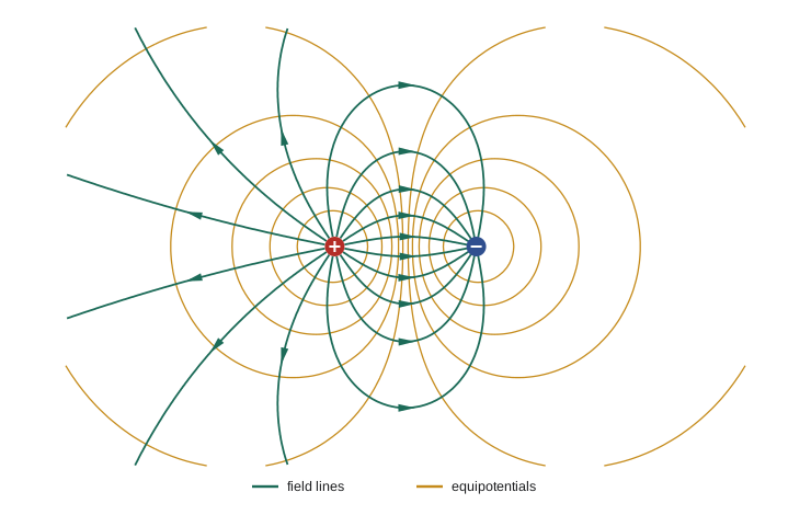
Equipotential surfaces, on which \(V\) is constant, are everywhere perpendicular to the field lines. For a point charge they are spheres; for a dipole, a pair of equal and opposite charges, they form the closed curves shown in the figure, surrounding each charge and becoming flattened between them. The plane midway between the charges is an equipotential at \(V = 0\). Field lines leave the positive charge at right angles to every equipotential they cross and converge on the negative charge.

Boundary conditions on the potential

The boundary condition on the field across a surface charge, derived in lesson 4, translates into conditions on the potential. The potential itself is continuous across any surface: since the field is finite, the line integral of \(\mathbf{E}\) across a layer of vanishing thickness is zero. Its normal derivative, however, jumps, because the normal field jumps:

These two conditions are what we impose when we solve Laplace's equation separately on the two sides of a charged surface and stitch the solutions together, as lesson 8 does for a sphere with a cosine surface charge. A useful way to picture them is a tent: the potential is a continuous surface whose slope changes abruptly along any line of surface charge, just as a tent fabric has a crease along its ridge pole.

Computing a potential and its field

The program computes the potential of a ring of radius 10 cm carrying 10 nC by summing \(k\,dq/\mathscr{r}\) over 2000 elements. It then finds the field on the axis by differentiating numerically, \(E_z = -\partial V/\partial z\), and compares with the exact on-axis formula \(E_z = kQz/(a^2 + z^2)^{3/2}\). Next it computes the energy needed to assemble four point charges, and finally it builds a uniformly charged sphere shell by shell, adding the work needed to bring each new shell in from infinity against the charge already present.

import math
k = 8.9875517923e9
# 1. Potential of a charged ring (radius a = 0.1 m, Q = 10 nC) by integration, and the
#    field from E = -grad V by finite differences, compared with the on-axis formula.
a, Q, N = 0.1, 10e-9, 2000
def V(x, z):                    # field point (x, 0, z); ring in the xy plane
    s = 0.0
    for i in range(N):
        ph = 2*math.pi*(i + .5)/N
        s += k*(Q/N)/math.sqrt((x - a*math.cos(ph))**2 + (a*math.sin(ph))**2 + z*z)
    return s
h = 1e-5
for z in (0.0, 0.05, 0.1, 0.3):
    Ez = -(V(0, z + h) - V(0, z - h))/(2*h)
    Ez = 0.0 if abs(Ez) < 1e-6 else Ez
    exact = k*Q*z/(a*a + z*z)**1.5
    print(f"axis z = {z:4.2f} m: V = {V(0, z):7.1f} V, Ez from -dV/dz = {Ez:8.1f}, formula {exact:8.1f} N/C")
Ex = -(V(0.05 + h, 0.02) - V(0.05 - h, 0.02))/(2*h)
print(f"off axis at (0.05, 0, 0.02): Ex = {Ex:.1f} N/C")

# 2. Energy of a configuration of point charges: W = (1/2) sum_i q_i V_i
qs = [(1e-9, (0, 0, 0)), (-2e-9, (0.1, 0, 0)), (3e-9, (0, 0.1, 0)), (-1e-9, (0.1, 0.1, 0.1))]
W = 0.0
for i, (qi, ri) in enumerate(qs):
    for j, (qj, rj) in enumerate(qs):
        if i < j: W += k*qi*qj/math.dist(ri, rj)
print(f"assembly energy of four charges: {W*1e9:.2f} nJ")

# 3. Self-energy of a uniformly charged sphere, built shell by shell: W -> (3/5) k Q^2 / R
R, Q = 0.1, 10e-9
for n in (10, 100, 1000):
    W = 0.0; q = 0.0
    for i in range(n):
        r = R*(i + .5)/n; dq = Q*3*r*r*(R/n)/R**3
        W += k*q*dq/r; q += dq
    print(f"{n:5d} shells: W = {W*1e6:.4f} uJ   (3/5 kQ^2/R = {0.6*k*Q*Q/R*1e6:.4f} uJ)")

axis z = 0.00 m: V =   898.8 V, Ez from -dV/dz =      0.0, formula      0.0 N/C
axis z = 0.05 m: V =   803.9 V, Ez from -dV/dz =   3215.5, formula   3215.5 N/C
axis z = 0.10 m: V =   635.5 V, Ez from -dV/dz =   3177.6, formula   3177.6 N/C
axis z = 0.30 m: V =   284.2 V, Ez from -dV/dz =    852.6, formula    852.6 N/C
off axis at (0.05, 0, 0.02): Ex = -2266.7 N/C
assembly energy of four charges: -406.88 nJ
   10 shells: W = 4.3865 uJ   (3/5 kQ^2/R = 5.3925 uJ)
  100 shells: W = 5.2914 uJ   (3/5 kQ^2/R = 5.3925 uJ)
 1000 shells: W = 5.3824 uJ   (3/5 kQ^2/R = 5.3925 uJ)

The potential at the center of the ring is \(kQ/a = 899\) V, since every element is the same distance away, but the field there is zero by symmetry: the potential is a maximum along the axis at the center. Differentiating the potential numerically reproduces the field formula to all printed digits at every height, and the field is largest near \(z = a/\sqrt2 \approx 7\) cm. Off the axis the program finds a field of 2267 N/C pointing inward toward the axis at a point inside the ring, something that would be laborious to obtain from Coulomb's law by hand but costs nothing once \(V\) is known. The four-charge assembly energy is negative, \(-407\) nJ: the configuration is bound, and work would have to be done to pull it apart. The shell-by-shell construction converges toward \(\frac35 kQ^2/R = 5.39\) μJ as the shells become thinner.

The energy of a charge distribution

Bringing a charge \(q\) from infinity to a point where the potential is \(V\) takes work \(qV\). Assembling a set of point charges one at a time therefore takes

where \(V(\mathbf{r}_i)\) is the potential at charge \(i\) due to all the others; the factor of one half corrects for counting each pair twice. For a continuous distribution the sum becomes \(W = \frac12\int\rho V\,d\tau\). Replacing \(\rho\) by \(\varepsilon_0\nabla\cdot\mathbf{E}\), integrating by parts with the product rule, and letting the volume grow to include all space so that the surface term vanishes, gives

This remarkable formula says that the energy can be regarded as stored in the field, with energy density \(\varepsilon_0 E^2/2\), even in empty space far from any charge. For a uniformly charged sphere it gives \(W = \frac35\,Q^2/(4\pi\varepsilon_0 R)\), the result the program approaches.

Two subtleties deserve attention. First, the field-energy formula is always positive, but the point-charge sum can be negative. The difference is the self-energy of each point charge, the energy needed to assemble the point charge itself, which is infinite for a true point. The sum over pairs leaves those infinite constants out; the field formula includes them. For ordinary problems we only need energy differences, and the infinities cancel. Second, energy is not additive under superposition: the energy of two fields together is \(\frac{\varepsilon_0}{2}\int(\mathbf{E}_1 + \mathbf{E}_2)^2\,d\tau\), which includes a cross term \(\varepsilon_0\int\mathbf{E}_1\cdot\mathbf{E}_2\,d\tau\). That cross term is the interaction energy.

Setting the self-energy \(\frac35 e^2/(4\pi\varepsilon_0 R)\) of a sphere of charge equal to the rest energy \(m_e c^2\) of an electron gives a radius of about a femtometre. Its close cousin, \(e^2/(4\pi\varepsilon_0 m_e c^2) = 2.82 \times 10^{-15}\) m, is called the classical electron radius. It is not the size of the electron, which behaves as a point particle in every experiment so far, but it marks the scale at which classical electrodynamics must give way to quantum field theory.