Vector calculus for electromagnetism: gradient, divergence, curl and the theorems

Electromagnetic theory is written in the language of vector calculus. The multivariable calculus course introduced the operators and the integral theorems; this lesson collects them in the form physicists use, explains what each one measures, proves the key identities and checks the two great theorems numerically. Everything here will be used repeatedly: the gradient connects the potential to the field, the divergence measures sources, the curl measures circulation, and the divergence and Stokes theorems turn local differential laws into the integral laws you can apply to Gaussian surfaces and Amperian loops.

The del operator

In Cartesian coordinates the vector differential operator del is

It is not a vector in the ordinary sense, because it has no value until it acts on something, but it behaves like one in many formulas. It can act in three ways. On a scalar function \(T\) it gives the gradient \(\nabla T\), a vector. Dotted into a vector function \(\mathbf{v}\) it gives the divergence \(\nabla\cdot\mathbf{v}\), a scalar. Crossed with \(\mathbf{v}\) it gives the curl \(\nabla\times\mathbf{v}\), a vector. There is no fourth first-derivative operation: these three exhaust the ways of combining a vector operator with a scalar or a vector.

The gradient

For a scalar function \(T(x, y, z)\), the change in \(T\) when we move by a small displacement \(d\mathbf{l} = (dx, dy, dz)\) is

For a step of fixed length, \(dT\) is largest when \(d\mathbf{l}\) points along \(\nabla T\). So the gradient points in the direction of steepest increase, and its magnitude is the rate of increase in that direction. It is perpendicular to the level surfaces of \(T\), because moving along a level surface does not change \(T\). Integrating \(dT\) along any path gives the fundamental theorem for gradients,

so the line integral of a gradient depends only on the end points, and around any closed loop it is zero. In electrostatics the field is minus the gradient of the potential, \(\mathbf{E} = -\nabla V\), so the field points from high potential to low, crosses equipotential surfaces at right angles, and does no net work on a charge taken around a closed path.

The divergence

The divergence of \(\mathbf{v} = (v_x, v_y, v_z)\) is

It measures how much the field spreads out from a point. Picture \(\mathbf{v}\) as the velocity of a fluid. If more fluid leaves a small box than enters it, there must be a source inside, and the divergence is positive. To see this, take a tiny box with sides \(dx\), \(dy\), \(dz\). The net outward flow through the two faces perpendicular to \(x\) is \([v_x(x + dx) - v_x(x)]\,dy\,dz = (\partial v_x/\partial x)\,d\tau\), where \(d\tau = dx\,dy\,dz\). Adding the other two pairs of faces gives a net outward flux of \((\nabla\cdot\mathbf{v})\,d\tau\). The divergence is outward flux per unit volume. In electrostatics, \(\nabla\cdot\mathbf{E} = \rho/\varepsilon_0\): electric field spreads out from positive charge and converges on negative charge, and in empty space it has zero divergence.

The curl

The curl of \(\mathbf{v}\) is

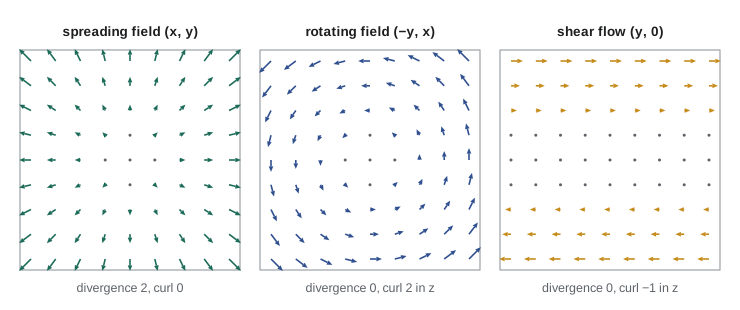
It measures how much the field circulates around a point. If you placed a tiny paddle wheel in the fluid, the curl would point along the axis about which the wheel turns fastest, with a magnitude equal to twice its angular velocity. Applying the same box argument to a small rectangle in the xy plane, the circulation \(\oint \mathbf{v}\cdot d\mathbf{l}\) around it is \((\partial v_y/\partial x - \partial v_x/\partial y)\,dx\,dy\), the z component of the curl times the area. The curl is circulation per unit area. A field can circulate without visibly swirling: a shear flow such as \(\mathbf{v} = (y, 0, 0)\), where the fluid moves faster higher up, turns a paddle wheel even though every streamline is straight.

Product rules and second derivatives

Because \(\nabla\) is a differential operator, products obey versions of the product rule, for example

Each can be verified by writing out components. Applying \(\nabla\) twice gives five combinations, of which two always vanish. The curl of a gradient is zero, \(\nabla\times(\nabla T) = \mathbf{0}\), because mixed partial derivatives are equal: the z component is \(\partial^2 T/\partial x\partial y - \partial^2 T/\partial y\partial x = 0\). The divergence of a curl is zero, \(\nabla\cdot(\nabla\times\mathbf{v}) = 0\), for the same reason. The divergence of a gradient is the Laplacian,

which will dominate lessons 7 and 8. The remaining combination is the curl of a curl, \(\nabla\times(\nabla\times\mathbf{v}) = \nabla(\nabla\cdot\mathbf{v}) - \nabla^2\mathbf{v}\), which is how the wave equation emerges from Maxwell's equations. The two vanishing identities have important converses, proved in more advanced courses: a field with zero curl everywhere is the gradient of a scalar, and a field with zero divergence everywhere is the curl of a vector. The first gives us the electric potential; the second gives us the magnetic vector potential of lesson 11.

The divergence theorem

The divergence theorem, associated with Gauss, Ostrogradsky and Green, states that for a volume \(\mathcal{V}\) bounded by a closed surface \(\mathcal{S}\) with outward normal,

The proof is the box argument extended: divide the volume into tiny cubes. For each cube, the divergence times its volume equals its net outward flux. When the cubes are added, the flux through every interior face is counted twice with opposite signs and cancels, leaving only the flux through the outer surface. The total of the sources inside equals the net flow out through the boundary. Applied to the electric field, it converts \(\nabla\cdot\mathbf{E} = \rho/\varepsilon_0\) into Gauss's law, \(\oint \mathbf{E}\cdot d\mathbf{a} = Q_{\text{enc}}/\varepsilon_0\).

Stokes' theorem

Stokes' theorem relates the curl over a surface \(\mathcal{S}\) to the circulation around its boundary curve \(\mathcal{P}\):

The directions are linked by the right-hand rule: if your fingers follow the boundary, your thumb gives the direction of \(d\mathbf{a}\). The proof again tiles the surface with small patches; the circulation around each patch is its curl times its area, and interior edges cancel. Two consequences are worth noting. The left side depends only on the boundary, not on which surface you choose, so the flux of a curl through any surface bounded by the same loop is the same. And the flux of a curl through a closed surface, which has no boundary, is zero. Applied to the magnetic field, Stokes' theorem turns \(\nabla\times\mathbf{B} = \mu_0\mathbf{J}\) into Ampère's law, \(\oint\mathbf{B}\cdot d\mathbf{l} = \mu_0 I_{\text{enc}}\).

Checking the theorems numerically

The program computes divergence and curl by central differences, \(\partial f/\partial x \approx [f(x + h) - f(x - h)]/2h\), for three fields at the point (1, 2, 0.5). The first is \(\mathbf{F}_1 = (y^2,\ 2xy + z^2,\ 2yz)\), the second a pure rotation and the third a pure spreading. It then checks the divergence theorem for \(\mathbf{F}_1\) on the unit cube by computing the volume integral of the divergence with a 40 by 40 by 40 grid of midpoints and, separately, the flux through the six faces. Finally it checks Stokes' theorem for the rotating field around a circle of radius 2.

import math
# Numerical divergence and curl on a grid by central differences, and checks of the
# divergence theorem and Stokes' theorem for sample fields.
h = 1e-4
def div(F, x, y, z):
    return ((F(x+h, y, z)[0] - F(x-h, y, z)[0]) + (F(x, y+h, z)[1] - F(x, y-h, z)[1])
            + (F(x, y, z+h)[2] - F(x, y, z-h)[2])) / (2*h)
def curl(F, x, y, z):
    d = lambda i, j: (F(*[c + (h if n == j else 0) for n, c in enumerate((x, y, z))])[i]
                     - F(*[c - (h if n == j else 0) for n, c in enumerate((x, y, z))])[i]) / (2*h)
    return (d(2, 1) - d(1, 2), d(0, 2) - d(2, 0), d(1, 0) - d(0, 1))

F1 = lambda x, y, z: (y*y, 2*x*y + z*z, 2*y*z)    # a textbook field
F2 = lambda x, y, z: (-y, x, 0.0)                  # pure rotation
F3 = lambda x, y, z: (x, y, z)                     # pure spreading
p = (1.0, 2.0, 0.5)
for name, F in (("F1", F1), ("F2", F2), ("F3", F3)):
    c = curl(F, *p)
    print(f"{name}: div = {div(F, *p)+0:7.3f}   curl = ({c[0]+0:6.3f}, {c[1]+0:6.3f}, {c[2]+0:6.3f})".replace("-0.000", " 0.000"))

# Divergence theorem for F1 on the unit cube [0,1]^3 (midpoint rule)
n = 40; dA = 1.0 / n**2; dV = 1.0 / n**3
vol = sum(div(F1, (i+.5)/n, (j+.5)/n, (l+.5)/n) * dV
          for i in range(n) for j in range(n) for l in range(n))
flux = 0.0
for i in range(n):
    for j in range(n):
        u, w = (i+.5)/n, (j+.5)/n
        flux += (F1(1, u, w)[0] - F1(0, u, w)[0]) * dA      # x faces
        flux += (F1(u, 1, w)[1] - F1(u, 0, w)[1]) * dA      # y faces
        flux += (F1(u, w, 1)[2] - F1(u, w, 0)[2]) * dA      # z faces
print(f"cube: volume integral of div F1 = {vol:.5f}, outward flux = {flux:.5f}")

# Stokes' theorem for F2 around a circle of radius 2 in the xy plane
N = 2000; circ = 0.0
for k in range(N):
    t = 2*math.pi*(k + .5)/N
    x, y = 2*math.cos(t), 2*math.sin(t)
    dx, dy = -2*math.sin(t)*2*math.pi/N, 2*math.cos(t)*2*math.pi/N
    Fx, Fy, _ = F2(x, y, 0)
    circ += Fx*dx + Fy*dy
print(f"circle r=2: circulation = {circ:.5f}, (curl F2)_z times area = {2*math.pi*4:.5f}")

F1: div =   6.000   curl = ( 0.000,  0.000,  0.000)
F2: div =   0.000   curl = ( 0.000,  0.000,  2.000)
F3: div =   3.000   curl = ( 0.000,  0.000,  0.000)
cube: volume integral of div F1 = 2.00000, outward flux = 2.00000
circle r=2: circulation = 25.13274, (curl F2)_z times area = 25.13274

For \(\mathbf{F}_1\), the divergence is \(2x + 2y = 6\) at the test point and its curl is zero everywhere: it is the gradient of \(xy^2 + yz^2\), so the identity \(\nabla\times\nabla T = \mathbf{0}\) shows up numerically. The volume integral of \(2x + 2y\) over the unit cube is exactly 2, and the six face fluxes add to the same 2 to five decimal places. The midpoint rule happens to be exact here because the integrand is linear. The rotating field \((-y, x, 0)\) has curl 2 in the z direction everywhere, so its flux through a disc of radius 2 is \(2 \times 4\pi = 25.13\), and the circulation around the boundary circle agrees. The pure spreading field \((x, y, z)\) has divergence 3, the number of dimensions, and no curl.