The vector potential and magnetic boundary conditions

In electrostatics the zero curl of \(\mathbf{E}\) let us write it as the gradient of a scalar potential. In magnetostatics it is the zero divergence of \(\mathbf{B}\) that lets us write it as the curl of a vector potential, \(\mathbf{B} = \nabla\times\mathbf{A}\). The vector potential is less intuitive than \(V\), but it is just as useful: it turns Ampère's law into three copies of Poisson's equation, it gives a compact formula for the field of any current distribution, it provides an elegant way to compute magnetic flux, and in quantum mechanics and relativity it turns out to be more fundamental than \(\mathbf{B}\) itself. This lesson introduces \(\mathbf{A}\), discusses the freedom in choosing it, derives the boundary conditions on \(\mathbf{B}\) at a current sheet, and develops the multipole expansion for magnetic fields, whose leading term is the magnetic dipole.

Defining the vector potential

Because the divergence of any curl is zero, setting \(\mathbf{B} = \nabla\times\mathbf{A}\) automatically satisfies \(\nabla\cdot\mathbf{B} = 0\). The other field equation then becomes

The vector potential is not unique. Adding the gradient of any scalar function, \(\mathbf{A} \to \mathbf{A} + \nabla\lambda\), leaves \(\mathbf{B}\) unchanged, because the curl of a gradient vanishes. This freedom, called gauge freedom, lets us impose one extra condition for convenience. In magnetostatics the standard choice is the Coulomb gauge, \(\nabla\cdot\mathbf{A} = 0\). It can always be achieved: if some \(\mathbf{A}_0\) has nonzero divergence, choosing \(\lambda\) to solve \(\nabla^2\lambda = -\nabla\cdot\mathbf{A}_0\), which is Poisson's equation with a known source, removes it. With the Coulomb gauge, the field equation becomes

three Poisson equations, one for each Cartesian component. We already know the solution of Poisson's equation from electrostatics, with \(\rho/\varepsilon_0\) replaced by \(\mu_0\mathbf{J}\). For currents confined to a finite region,

This formula is often easier to use than Biot–Savart because it has no cross product: \(\mathbf{A}\) points in the same direction as the current that produces it, weighted by \(1/\mathscr{r}\). For example, the vector potential of a current along \(z\) points along \(z\), and the vector potential of a circular loop circles the axis like the current. Taking the curl recovers the Biot–Savart law.

Flux and circulation

The vector potential gives a neat way to compute magnetic flux. By Stokes' theorem, the flux of \(\mathbf{B}\) through any surface \(\mathcal{S}\) equals the circulation of \(\mathbf{A}\) around its boundary:

This is formally the same as Ampère's law with \(\mathbf{A}\) in place of \(\mathbf{B}\) and \(\Phi\) in place of \(\mu_0I\), so symmetric problems can be solved the same way. For a long solenoid of radius \(R\) with uniform internal field \(B = \mu_0nI\), a circle of radius \(s\) around the axis gives \(A_\phi\cdot 2\pi s = \pi s^2B\) inside and \(\pi R^2B\) outside:

Outside the solenoid \(\mathbf{B}\) is zero but \(\mathbf{A}\) is not. Classically this makes no difference, since forces depend only on \(\mathbf{B}\). In quantum mechanics it matters: Yakir Aharonov and David Bohm predicted in 1959 that electrons passing on either side of a solenoid, through regions where \(\mathbf{B} = 0\), acquire a phase difference proportional to the enclosed flux, and experiments, most cleanly Tonomura's in 1986, confirmed the effect. The vector potential, or more precisely its circulation, is physically real.

Contours of A as field lines

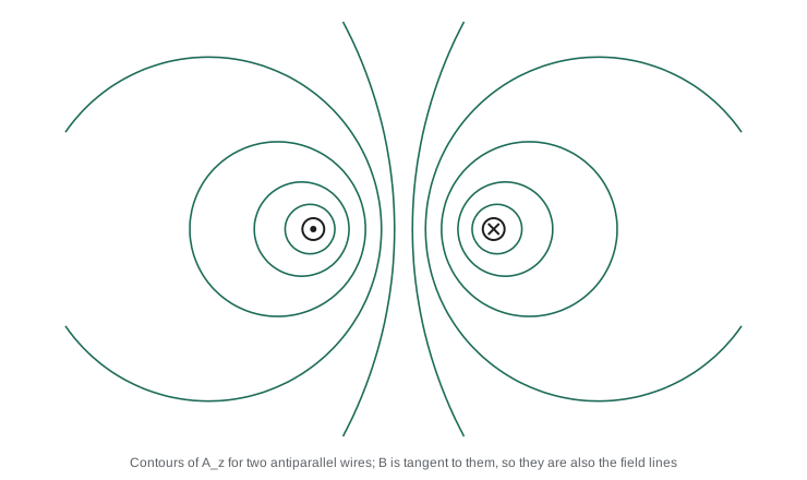
In two-dimensional problems, where all currents run parallel to the z axis and nothing depends on \(z\), \(\mathbf{A} = A_z(x, y)\hat{\mathbf{z}}\) and

This vector is perpendicular to \(\nabla A_z\), so it is tangent to the contours of \(A_z\). The contours of \(A_z\) are the field lines, and the flux between two contours per unit length equals the difference of their \(A_z\) values. This is how electrical engineers draw the fields of transmission lines, motors and transformers in two-dimensional finite-element programs. The figure shows the case of two long antiparallel wires, a model of a two-wire power cord, for which \(A_z \propto \ln(s_2/s_1)\), where \(s_1\) and \(s_2\) are the distances to the two wires.

Boundary conditions for B

At a surface carrying a surface current \(\mathbf{K}\), the field changes abruptly. A flat pillbox straddling the surface has no net flux because \(\nabla\cdot\mathbf{B} = 0\), so the normal component is continuous. A thin rectangular Amperian loop crossing the surface perpendicular to the current encloses current \(K\,l\), so the tangential component perpendicular to \(\mathbf{K}\) jumps by \(\mu_0K\). Together,

where \(\hat{\mathbf{n}}\) points from below to above. These mirror the electric conditions, with the roles of the normal and tangential components exchanged. The vector potential, by contrast, is continuous across any surface current, though its normal derivative jumps by \(-\mu_0\mathbf{K}\).

The magnetic multipole expansion

Far from a localized current distribution, expand \(1/\mathscr{r}\) in Legendre polynomials exactly as in lesson 8. For a current loop,

The monopole term \(\oint d\mathbf{l}'\) is always zero, because the loop closes: there is no magnetic monopole. The leading term is the dipole,

where \(\mathbf{m}\) is the magnetic dipole moment, the current times the vector area of the loop. Its field,

has the same form as the electric dipole field far away, although near the source the two are different: inside a current loop the field points along \(\mathbf{m}\), while between two separated charges the field points opposite to \(\mathbf{p}\). The Earth's field is, to a first approximation, that of a magnetic dipole of moment about \(8 \times 10^{22}\) A m\(^2\), tilted about 10 degrees from the rotation axis, produced by currents in the liquid iron outer core.

The magnetic dipole also has a simple energy and torque. In a uniform external field it feels a torque \(\mathbf{N} = \mathbf{m}\times\mathbf{B}\) that tends to align \(\mathbf{m}\) with \(\mathbf{B}\), and it has energy \(U = -\mathbf{m}\cdot\mathbf{B}\), lowest when aligned. These formulas, identical in form to the electric ones, explain how a compass needle works, how an electric motor produces torque, and why atomic magnetic moments line up in a field, the starting point of the next lesson.

Computing A and the flux

The program computes the vector potential of a current loop by integrating \(\cos\phi'/\mathscr{r}\) around it, then evaluates its circulation around a tiny circle of radius 1 mm centered on the axis, which by Stokes' theorem equals the flux, and divides by the area to recover \(B_z\). It then tabulates \(B\) and \(A_\phi\) for a long solenoid of radius 2 cm with 2000 turns per meter carrying 2 A, checks the boundary condition at a current sheet of 50 A/m, and finally evaluates the dipole field of the Earth at the surface as a function of magnetic latitude.

import math
mu0 = 4e-7*math.pi
# 1. Vector potential of a current loop: A_phi(s, z) = (mu0 I a / 4 pi) * integral of cos(phi') / |r - r'| dphi'.
#    Check that B_z on the axis follows from the flux of B through a disc = circulation of A.
a, I = 0.1, 10.0
def A_phi(s, z, n=4000):
    tot = 0.0
    for i in range(n):
        ph = 2*math.pi*(i + .5)/n
        d = math.sqrt(s*s + a*a - 2*s*a*math.cos(ph) + z*z)
        tot += math.cos(ph)/d*2*math.pi/n
    return mu0*I*a/(4*math.pi)*tot
for z in (0.0, 0.1):
    s = 1e-3
    flux_from_A = 2*math.pi*s*A_phi(s, z)            # circulation of A round a small circle of radius s
    Bz = mu0*I*a*a/(2*(a*a + z*z)**1.5)
    print(f"z = {z:.2f} m: circulation of A / (pi s^2) = {flux_from_A/(math.pi*s*s)*1e6:.3f} uT, "
          f"axial B = {Bz*1e6:.3f} uT")

# 2. Long solenoid (n = 2000 turns per m, I = 2 A, radius R = 2 cm): B inside, A outside.
n_t, I_s, R = 2000, 2.0, 0.02
B_in = mu0*n_t*I_s
for s in (0.01, 0.015, 0.04, 0.10):
    A = mu0*n_t*I_s*s/2 if s < R else mu0*n_t*I_s*R*R/(2*s)
    print(f"s = {s:.3f} m: B = {(B_in if s < R else 0.0)*1e3:6.3f} mT, A_phi = {A*1e6:7.3f} uT m, "
          f"2 pi s A_phi = {2*math.pi*s*A*1e6:7.4f} uWb (enclosed flux)")

# 3. Boundary conditions at a current sheet K = 50 A/m in the plane z = 0 (flowing along x):
#    tangential B jumps by mu0 K, normal B is continuous.
K = 50.0
above, below = (0.0, -mu0*K/2), (0.0, +mu0*K/2)   # (B_x, B_y) just above and just below
print(f"current sheet: B_y above {above[1]*1e6:.2f} uT, below {below[1]*1e6:.2f} uT, "
      f"jump {abs(above[1] - below[1])*1e6:.2f} uT = mu0 K = {mu0*K*1e6:.2f} uT")

# 4. Earth's magnetic dipole: m = 8.0e22 A m^2. Field at the surface at magnetic latitude lam:
m, RE = 8.0e22, 6.371e6
for lam in (0, 30, 50, 60, 90):
    B = mu0*m/(4*math.pi*RE**3)*math.sqrt(1 + 3*math.sin(math.radians(lam))**2)
    dip = math.degrees(math.atan(2*math.tan(math.radians(lam))))
    print(f"magnetic latitude {lam:2d} deg: |B| = {B*1e6:5.1f} uT, dip angle {dip:4.1f} deg")

z = 0.00 m: circulation of A / (pi s^2) = 62.834 uT, axial B = 62.832 uT
z = 0.10 m: circulation of A / (pi s^2) = 22.214 uT, axial B = 22.214 uT
s = 0.010 m: B =  5.027 mT, A_phi =  25.133 uT m, 2 pi s A_phi =  1.5791 uWb (enclosed flux)
s = 0.015 m: B =  5.027 mT, A_phi =  37.699 uT m, 2 pi s A_phi =  3.5531 uWb (enclosed flux)
s = 0.040 m: B =  0.000 mT, A_phi =  25.133 uT m, 2 pi s A_phi =  6.3165 uWb (enclosed flux)
s = 0.100 m: B =  0.000 mT, A_phi =  10.053 uT m, 2 pi s A_phi =  6.3165 uWb (enclosed flux)
current sheet: B_y above -31.42 uT, below 31.42 uT, jump 62.83 uT = mu0 K = 62.83 uT
magnetic latitude  0 deg: |B| =  30.9 uT, dip angle  0.0 deg
magnetic latitude 30 deg: |B| =  40.9 uT, dip angle 49.1 deg
magnetic latitude 50 deg: |B| =  51.4 uT, dip angle 67.2 deg
magnetic latitude 60 deg: |B| =  55.8 uT, dip angle 73.9 deg
magnetic latitude 90 deg: |B| =  61.9 uT, dip angle 90.0 deg

The circulation of \(\mathbf{A}\) reproduces the axial field of the loop to four figures. For the solenoid, \(A_\phi\) grows linearly inside, peaks at the winding, and then falls as \(1/s\) outside, where \(\mathbf{B}\) vanishes; the circulation \(2\pi sA_\phi\) outside is constant at 6.32 μWb, the flux trapped in the solenoid. At the current sheet, \(B_y\) flips sign across the sheet and jumps by \(\mu_0K = 62.8\) μT. The Earth's dipole field rises from 31 μT at the magnetic equator to 62 μT at the magnetic poles. At magnetic latitude 60 degrees, roughly that of the Canadian prairies and the upper Midwest, the dipole model gives about 56 μT and a dip angle of 74 degrees: compass needles there point steeply downward, which is why navigation compasses are balanced for the latitude where they are sold. Real values differ by a few microteslas because the Earth's field is not a pure dipole, and the magnetic poles drift; the north magnetic pole has moved from northern Canada toward Siberia over the past century.