Electrostatics: Coulomb's law, Gauss's law and the electric field

With the mathematical tools in place, we turn to electrostatics proper. This lesson derives the two field equations of electrostatics, \(\nabla\cdot\mathbf{E} = \rho/\varepsilon_0\) and \(\nabla\times\mathbf{E} = \mathbf{0}\), directly from Coulomb's law and superposition, shows how Gauss's law in integral form follows, and uses it to find the fields of the standard symmetric distributions. It also explains carefully when Gauss's law is useful and when it is not. Gauss's law is always true, but it gives the field only when symmetry lets us pull \(|\mathbf{E}|\) out of the flux integral.

The divergence of the electric field

Start from the field of a continuous charge distribution,

Take the divergence with respect to the field point \(\mathbf{r}\). The charge density depends only on the source point, so the divergence acts only on \(\hat{\boldsymbol{\mathscr{r}}}/\mathscr{r}^2\), which by lesson 3 gives \(4\pi\delta^3(\mathbf{r} - \mathbf{r}')\). The delta function then collapses the integral:

This is Gauss's law in differential form. It says that the divergence of the electric field at a point is set by the charge density at that same point, and nowhere else. Charges elsewhere influence the field here, of course, but they contribute no divergence here. Integrating over any volume and applying the divergence theorem gives the integral form,

the statement Carl Friedrich Gauss formulated in work on magnetism and gravitation in the 1830s and published in 1867 in his collected works. The flux of \(\mathbf{E}\) through any closed surface equals the enclosed charge divided by \(\varepsilon_0\), whatever the shape of the surface and wherever the charges inside sit.

The curl of the electric field

For a point charge at the origin, \(\mathbf{E}\) is radial, and its line integral from \(\mathbf{a}\) to \(\mathbf{b}\) is

because only the radial part of \(d\mathbf{l}\), namely \(dr\), contributes. The result depends only on the end points, so around any closed loop the integral is zero. By superposition the same holds for any static charge distribution, and Stokes' theorem then gives

An electrostatic field has no circulation. This is what makes the scalar potential of lesson 5 possible. It is also a strong constraint: a field such as \(k(y\,\hat{\mathbf{x}} - x\,\hat{\mathbf{y}})\), however tidy it looks, can never be produced by any arrangement of static charges, because its curl is not zero. The curl condition fails when magnetic fields change with time, which is Faraday's law and the subject of PHYS-382.

Using Gauss's law

Gauss's law is a powerful way to compute fields, but only for three kinds of symmetry: spherical, cylindrical and planar. In each case we choose a Gaussian surface on which \(\mathbf{E}\) is either perpendicular to the surface with constant magnitude, or parallel to it so that it contributes no flux. Then the flux integral reduces to \(|\mathbf{E}|\) times an area. The arguments rely on symmetry to fix the direction of \(\mathbf{E}\) before the law is applied: a spherically symmetric charge cannot produce a field with a preferred tangential direction, a long uniform line charge cannot produce a field with a component along the line, and so on.

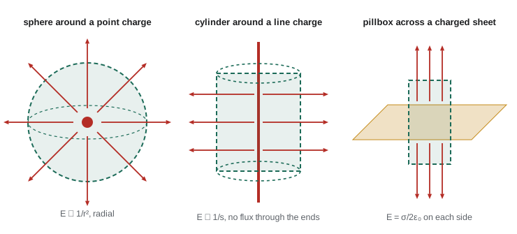
For a uniformly charged solid sphere of radius \(R\) and total charge \(Q\), choose a concentric sphere of radius \(r\). Outside the charge, \(E\cdot 4\pi r^2 = Q/\varepsilon_0\), so the field is exactly that of a point charge at the center. Inside, the enclosed charge is \(Q r^3/R^3\), so

For an infinite line charge \(\lambda\), a coaxial cylinder of radius \(s\) and length \(l\) has flux \(E\cdot 2\pi s l\) through its curved side and none through its ends, giving \(E = \lambda/(2\pi\varepsilon_0 s)\). For an infinite plane with surface charge \(\sigma\), a pillbox of area \(A\) has flux \(2EA\), giving \(E = \sigma/(2\varepsilon_0)\) on each side, independent of distance. These three results, falling off as \(1/r^2\), \(1/s\) and not at all, reflect how quickly the field lines spread in three, two and one dimensions.

Checking Gauss's law numerically

The program first estimates the flux of a 1 nC point charge through a sphere of radius 1 m by Monte Carlo integration: it chooses 200,000 random points uniformly on the sphere, averages \(\mathbf{E}\cdot\hat{\mathbf{n}}\) over them and multiplies by the area. It does this with the charge at the center, moved off-center, and placed outside the sphere. Next it builds the field of a uniformly charged solid sphere by adding the fields of 400 thin concentric shells, using only the fact that a shell acts as a point charge outside itself and produces no field inside. Finally it integrates the field of a finite line of charge 2 m long and compares it with the infinite-line and point-charge formulas.

import math, random
k = 8.9875517923e9
rnd = random.Random(381)
# 1. Gauss's law by Monte Carlo: flux of a point charge through a sphere of radius 1 m.
#    Points are spread uniformly over the sphere; the charge sits off the middle or outside.
def mc_flux(q, pos, R=1.0, n=200000):
    tot = 0.0
    for _ in range(n):
        z = 2*rnd.random() - 1; ph = 2*math.pi*rnd.random(); s = math.sqrt(1 - z*z)
        nx, ny, nz = s*math.cos(ph), s*math.sin(ph), z
        dx, dy, dz = R*nx - pos[0], R*ny - pos[1], R*nz - pos[2]
        r3 = (dx*dx + dy*dy + dz*dz)**1.5
        tot += k*q*(dx*nx + dy*ny + dz*nz)/r3
    return tot/n * 4*math.pi*R*R
eps0 = 1/(4*math.pi*k); q = 1e-9
for pos in ((0, 0, 0), (0.6, 0.3, 0.0), (1.5, 0.0, 0.0)):
    print(f"charge at {pos}: flux = {mc_flux(q, pos):8.2f} N m^2/C   (q/eps0 = {q/eps0:.2f})")

# 2. Field of a uniformly charged solid sphere (R = 0.1 m, Q = 5 nC) by direct integration
#    over shells, compared with Gauss's law: inside E grows linearly, outside like 1/r^2.
R, Q = 0.1, 5e-9; rho = Q/(4/3*math.pi*R**3)
def E_direct(r, n=400):
    # sum the fields of thin shells; a shell of radius s contributes kq/r^2 only if s < r
    tot = 0.0
    for i in range(n):
        s = R*(i + .5)/n; dq = rho*4*math.pi*s*s*R/n
        if s < r: tot += k*dq/r**2
    return tot
for r in (0.02, 0.05, 0.1, 0.2, 0.4):
    gauss = k*Q*r/R**3 if r < R else k*Q/r**2
    print(f"r = {r:4.2f} m: shell sum {E_direct(r):9.1f} N/C, Gauss {gauss:9.1f} N/C")

# 3. A finite line of charge (lambda = 2 nC/m, length 2 m): field at distance d from its midpoint
lam, Lh = 2e-9, 1.0
for d in (0.05, 0.5, 5.0):
    N = 20000; Ex = sum(k*lam*(2*Lh/N)*d/((-Lh + 2*Lh*(i+.5)/N)**2 + d*d)**1.5 for i in range(N))
    print(f"d = {d:4.2f} m: E = {Ex:9.2f} N/C; infinite line {2*k*lam/d:9.2f}; point charge {k*lam*2*Lh/d**2:9.2f}")

charge at (0, 0, 0): flux =   112.94 N m^2/C   (q/eps0 = 112.94)
charge at (0.6, 0.3, 0.0): flux =   112.88 N m^2/C   (q/eps0 = 112.94)
charge at (1.5, 0.0, 0.0): flux =    -0.01 N m^2/C   (q/eps0 = 112.94)
r = 0.02 m: shell sum     898.7 N/C, Gauss     898.8 N/C
r = 0.05 m: shell sum    2246.9 N/C, Gauss    2246.9 N/C
r = 0.10 m: shell sum    4493.8 N/C, Gauss    4493.8 N/C
r = 0.20 m: shell sum    1123.4 N/C, Gauss    1123.4 N/C
r = 0.40 m: shell sum     280.9 N/C, Gauss     280.9 N/C
d = 0.05 m: E =    718.11 N/C; infinite line    719.00; point charge  14380.08
d = 0.50 m: E =     64.31 N/C; infinite line     71.90; point charge    143.80
d = 5.00 m: E =      1.41 N/C; infinite line      7.19; point charge      1.44

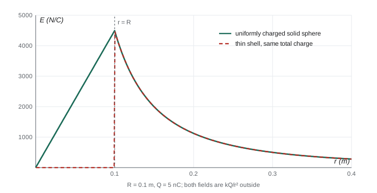
The flux is \(q/\varepsilon_0 = 112.9\) N m\(^2\)/C whenever the charge is inside, wherever it sits, and essentially zero when it is outside: field lines that enter the sphere also leave it. The statistical error of the Monte Carlo estimate is about 0.1%, visible in the off-center value. The shell sum reproduces the Gauss's-law field of the solid sphere at every radius, rising linearly inside and falling as \(1/r^2\) outside, with a maximum of 4494 N/C at the surface. The finite line shows how the symmetric results are idealizations. Five centimeters from a 2 m rod the field is within 0.1% of the infinite-line value; at 50 cm the ends already matter and the field is 11% lower; at 5 m the rod looks like a point charge and the field is within 2% of \(kQ/d^2\).

When Gauss's law does not help

Gauss's law is true for every closed surface, including a cube around a point charge or a sphere around an off-center charge. But in those cases \(\mathbf{E}\) varies in direction and magnitude over the surface, so knowing the total flux does not tell us the field. Students sometimes try to apply Gauss's law to a finite cylinder or a square sheet; the symmetry arguments fail at the ends and edges, and so does the result. For such problems we must integrate Coulomb's law directly, use the potential, or solve Laplace's equation with boundary conditions, which is the subject of lessons 5 to 8. A useful trick sometimes rescues Gauss's law: a point charge at the corner of a cube sends exactly one eighth of its flux through the cube, because eight such cubes would surround it symmetrically. Of that flux, the three faces touching the corner receive none, and each of the other three receives \(q/(24\varepsilon_0)\).

Gauss's law and the gravitational analogy

Newton's law of gravity is also an inverse-square law, so it obeys a Gauss's law of its own: the flux of the gravitational field \(\mathbf{g}\) through a closed surface is \(-4\pi G M_{\text{enc}}\), the minus sign recording that gravity attracts. The famous results that took Newton years to prove in the Principia, that a spherical planet attracts as if all its mass were at its center and that a spherical shell exerts no force on anything inside it, follow in a line each from Gauss's law. The same argument gives the field inside a uniform planet, which falls linearly to zero at the center: an object dropped through a frictionless tunnel through the Earth would oscillate in simple harmonic motion with a period of about 84 minutes, the same as the period of a satellite skimming the surface.

The field at a surface charge

Gauss's law also tells us how the field changes across a surface carrying charge \(\sigma\). A thin pillbox straddling the surface has flux \((E^{\perp}_{\text{above}} - E^{\perp}_{\text{below}})A = \sigma A/\varepsilon_0\), so the normal component jumps by \(\sigma/\varepsilon_0\). A thin rectangular loop straddling the surface has zero circulation because \(\nabla\times\mathbf{E} = \mathbf{0}\), so the tangential component is continuous. Together,

where \(\hat{\mathbf{n}}\) points from below to above. This boundary condition is the key to conductors in lesson 6 and to dielectrics in lesson 9.