Magnetostatics: the Lorentz force, Biot–Savart and Ampère's law

Magnetostatics is the study of the fields produced by steady currents, currents that flow continuously without charge piling up anywhere. Its structure parallels electrostatics, with the Biot–Savart law in place of Coulomb's law and Ampère's law in place of Gauss's law, but the differences are as instructive as the similarities. Magnetic forces act only on moving charges and are always perpendicular to their velocity, so they do no work. Magnetic field lines have no ends. And the source of the field, current, is a vector rather than a scalar. This lesson develops the Lorentz force law, the Biot–Savart law and Ampère's law, and derives the two field equations of magnetostatics, \(\nabla\cdot\mathbf{B} = 0\) and \(\nabla\times\mathbf{B} = \mu_0\mathbf{J}\).

The Lorentz force

Hans Christian Ørsted discovered in 1820 that an electric current deflects a compass needle, the first link between electricity and magnetism. Within weeks André-Marie Ampère showed that two parallel currents attract and opposite currents repel. The modern statement is the Lorentz force law, named for Hendrik Lorentz, who wrote it in its present form in the 1890s: a charge \(q\) moving with velocity \(\mathbf{v}\) through fields \(\mathbf{E}\) and \(\mathbf{B}\) feels

The magnetic part is perpendicular to \(\mathbf{v}\), so it does no work: \(\mathbf{F}\cdot\mathbf{v} = 0\). Magnetic forces change the direction of a charge's motion but never its speed. In a uniform field a charge moves in a circle of radius \(R = mv/(qB)\) at the cyclotron frequency \(\omega = qB/m\), independent of speed, the principle Ernest Lawrence exploited in the cyclotron of 1931. With a component of velocity along the field the path becomes a helix, which is why charged particles from the Sun spiral along the Earth's field lines toward the polar regions and produce the aurora. When a magnetic force appears to do work, as when a magnet lifts a steel bar or a motor turns, the work is actually done by whatever maintains the currents, and the magnetic force merely redirects it.

For a current, the moving charges are replaced by a current element. A line current \(I\) flowing along \(d\mathbf{l}\) feels \(d\mathbf{F} = I\,d\mathbf{l}\times\mathbf{B}\); a surface current \(\mathbf{K}\) (current per unit width) feels \(\mathbf{K}\times\mathbf{B}\,da\); and a volume current density \(\mathbf{J}\) (current per unit area) feels \(\mathbf{J}\times\mathbf{B}\,d\tau\). Charge conservation requires the continuity equation \(\nabla\cdot\mathbf{J} = -\partial\rho/\partial t\), which for steady currents becomes \(\nabla\cdot\mathbf{J} = 0\): as much current flows out of any volume as in.

The Biot–Savart law

Jean-Baptiste Biot and Félix Savart measured the field of a long wire in 1820, and the law that bears their names gives the magnetic field of any steady current:

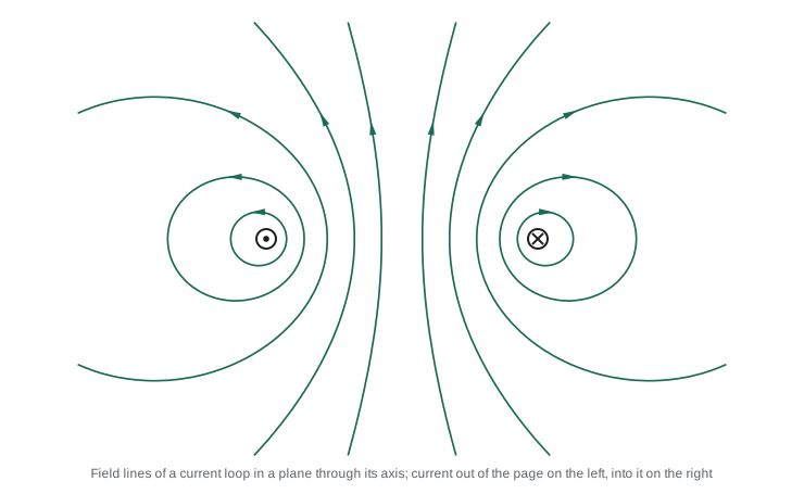
It plays the role of Coulomb's law: an inverse-square law with a cross product. For a long straight wire it gives \(B = \mu_0I/(2\pi s)\), circling the wire by the right-hand rule. For a circular loop of radius \(a\), on the axis at distance \(z\) from its center, only the axial components of the contributions survive, and

Far from the loop, \(B_z \approx \mu_0(I\pi a^2)/(2\pi z^3)\), the field of a magnetic dipole of moment \(m = I\pi a^2\). Two parallel wires a distance \(d\) apart, carrying currents \(I_1\) and \(I_2\), attract with a force per unit length \(\mu_0I_1I_2/(2\pi d)\). Until 2019 this was the definition of the ampere: the current that produces \(2 \times 10^{-7}\) N per meter between wires one meter apart.

The divergence and curl of B

Taking the divergence of the Biot–Savart law and using the identity \(\nabla\cdot(\mathbf{J}\times\hat{\boldsymbol{\mathscr{r}}}/\mathscr{r}^2) = \hat{\boldsymbol{\mathscr{r}}}/\mathscr{r}^2\cdot(\nabla\times\mathbf{J}) - \mathbf{J}\cdot\nabla\times(\hat{\boldsymbol{\mathscr{r}}}/\mathscr{r}^2)\), both terms vanish: \(\mathbf{J}\) depends on the source point, not the field point, and \(\hat{\boldsymbol{\mathscr{r}}}/\mathscr{r}^2\) is a gradient, so its curl is zero. Therefore

There are no magnetic charges; field lines never begin or end. Searches for magnetic monopoles, which some grand unified theories predict, have found none. Taking the curl instead, a longer calculation using the delta function and the steady-current condition \(\nabla\cdot\mathbf{J} = 0\) gives Ampère's law in differential form,

where the integral form follows from Stokes' theorem and \(I_{\text{enc}}\) is the current passing through any surface bounded by the loop. As in electrostatics, the two field equations together with a boundary condition at infinity determine \(\mathbf{B}\) uniquely.

Using Ampère's law

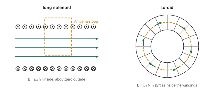
Ampère's law plays the role Gauss's law played in electrostatics. It always holds, but it yields the field only when symmetry tells us the direction of \(\mathbf{B}\) and lets us pull its magnitude out of the integral. The symmetric cases are infinite straight lines, infinite planes, infinite solenoids and toroids. For a long straight wire, a circular loop of radius \(s\) gives \(B\cdot 2\pi s = \mu_0I\). For a long solenoid with \(n\) turns per unit length, a rectangular loop with one side inside and one outside gives \(B = \mu_0nI\) inside, uniform, and zero outside. For a toroid with \(N\) turns, a circle of radius \(s\) inside the windings gives \(B = \mu_0NI/(2\pi s)\), and outside the toroid the field vanishes because the loop encloses zero net current. For an infinite plane of surface current \(\mathbf{K}\), the field is \(\mu_0K/2\), parallel to the plane and perpendicular to the current, pointing in opposite directions on the two sides.

Checking Biot–Savart and Ampère numerically

The program integrates the Biot–Savart law around a circular loop of radius 10 cm carrying 10 A, summing 2000 straight segments, and compares the axial field with the formula. Then it studies a Helmholtz pair, two coaxial loops whose separation equals their radius, a geometry Hermann von Helmholtz recommended for producing a uniform field. It compares the uniformity of the field near the middle for separations of half a radius, one radius and two radii. Finally it checks Ampère's law by integrating the field of a 5 A wire around a square that encloses the wire but is not centered on it, and computes the force between two 1 A wires one meter apart.

import math
mu0 = 4e-7*math.pi
# 1. Biot-Savart: field of a circular loop (radius a, current I) on its axis by summing
#    segments, compared with B = mu0 I a^2 / (2 (a^2 + z^2)^(3/2)).
def B_loop(x, y, z, a=0.1, I=10.0, n=2000, z0=0.0):
    Bx = By = Bz = 0.0
    for i in range(n):
        ph = 2*math.pi*(i + .5)/n; dph = 2*math.pi/n
        sx, sy, sz = a*math.cos(ph), a*math.sin(ph), z0
        dlx, dly = -a*math.sin(ph)*dph, a*math.cos(ph)*dph
        rx, ry, rz = x - sx, y - sy, z - sz
        r3 = (rx*rx + ry*ry + rz*rz)**1.5
        Bx += mu0*I/(4*math.pi)*(dly*rz)/r3            # dl x r with dl = (dlx, dly, 0)
        By += mu0*I/(4*math.pi)*(-dlx*rz)/r3
        Bz += mu0*I/(4*math.pi)*(dlx*ry - dly*rx)/r3
    return Bx, By, Bz
for z in (0.0, 0.05, 0.1, 0.3):
    exact = mu0*10.0*0.1**2/(2*(0.1**2 + z*z)**1.5)
    print(f"loop axis z = {z:4.2f} m: Biot-Savart {B_loop(0, 0, z)[2]*1e6:8.3f} uT, formula {exact*1e6:8.3f} uT")

# 2. Helmholtz pair: two loops separated by one radius give a very uniform field between them
a = 0.1
def Bz_pair(z, sep):
    return sum(mu0*10.0*a*a/(2*(a*a + (z - z0)**2)**1.5) for z0 in (-sep/2, sep/2))
for sep in (0.5*a, a, 2*a):
    B0 = Bz_pair(0, sep)
    dev = max(abs(Bz_pair(z, sep) - B0)/B0 for z in [i*0.002 for i in range(-10, 11)])
    print(f"separation {sep/a:.1f} a: B at the middle {B0*1e6:7.2f} uT, largest change within +/-2 cm "
          f"{dev*1e6:9.1f} parts per million")

# 3. Ampere's law: circulation of B around a long straight wire, on a circle and on a square
I = 5.0
B = lambda x, y: (-mu0*I/(2*math.pi)*y/(x*x + y*y), mu0*I/(2*math.pi)*x/(x*x + y*y))
N = 4000; circ = 0.0
for k in range(N):               # square of side 0.4 m, shifted sideways, enclosing the wire
    t = (k + .5)/N*4; side = int(t); u = t - side
    pts = [(-0.1, -0.15), (0.3, -0.15), (0.3, 0.25), (-0.1, 0.25), (-0.1, -0.15)]
    (x1, y1), (x2, y2) = pts[side], pts[side + 1]
    x, y = x1 + (x2 - x1)*u, y1 + (y2 - y1)*u
    Bx, By = B(x, y); circ += (Bx*(x2 - x1) + By*(y2 - y1))*4/N
print(f"square loop around a {I} A wire: circulation {circ:.6e} T m, mu0 I = {mu0*I:.6e} T m")
# 4. Force per unit length between two parallel wires 1 m apart carrying 1 A (the pre-2019 ampere definition)
print(f"force per unit length between 1 A wires 1 m apart: {mu0*1*1/(2*math.pi*1):.3e} N/m")

loop axis z = 0.00 m: Biot-Savart   62.832 uT, formula   62.832 uT
loop axis z = 0.05 m: Biot-Savart   44.959 uT, formula   44.959 uT
loop axis z = 0.10 m: Biot-Savart   22.214 uT, formula   22.214 uT
loop axis z = 0.30 m: Biot-Savart    1.987 uT, formula    1.987 uT
separation 0.5 a: B at the middle  114.74 uT, largest change within +/-2 cm   39172.1 parts per million
separation 1.0 a: B at the middle   89.92 uT, largest change within +/-2 cm    1763.5 parts per million
separation 2.0 a: B at the middle   44.43 uT, largest change within +/-2 cm   44411.1 parts per million
square loop around a 5.0 A wire: circulation 6.283186e-06 T m, mu0 I = 6.283185e-06 T m
force per unit length between 1 A wires 1 m apart: 2.000e-07 N/m

The segment sum reproduces the axial formula to all printed digits, 62.8 μT at the center of the loop, comparable to the Earth's field. The Helmholtz comparison is striking. With the loops one radius apart, the field changes by only 0.18% within 2 cm of the middle; closer together or farther apart, the change is twenty times larger. The reason is that at that separation the second derivative of the field at the middle vanishes, along with the first and third by symmetry, so the first nonuniformity is fourth order. Helmholtz coils are used to cancel the Earth's field in laboratories and to calibrate magnetometers. The circulation around the off-center square is \(\mu_0I = 6.283 \times 10^{-6}\) T m to six figures: Ampère's law, like Gauss's law, does not care about the shape of the loop. The final line recovers the historical definition of the ampere.

Crossed electric and magnetic fields give a useful device. A charge moving perpendicular to both \(\mathbf{E}\) and \(\mathbf{B}\), with \(\mathbf{E}\) perpendicular to \(\mathbf{B}\), feels no net force when \(qE = qvB\), that is when \(v = E/B\), independent of its charge and mass. A region of crossed fields therefore acts as a velocity selector: only particles with that speed pass straight through. Following it with a region of pure magnetic field, where each particle moves on a circle of radius \(mv/(qB)\), separates particles by their mass-to-charge ratio. This is the principle of the mass spectrometer, used to identify molecules in chemistry and medicine and to measure isotope ratios for radiometric dating.