The hydrogen atom: Bohr model, quantum numbers and spectra

Hydrogen, one proton and one electron, is the simplest atom and the most abundant element in the universe. It was the testing ground for every stage of quantum theory. In 1913 Niels Bohr, a young Danish physicist working with Rutherford in Manchester, built a model of hydrogen that combined Rutherford's nucleus with Planck's quanta and reproduced the Rydberg formula of lesson 1. Bohr's model was soon superseded, but its central idea of stationary states and quantum jumps survived. In 1926 Schrödinger solved his equation for hydrogen exactly, giving the same energy levels and much more: the shapes of the electron clouds, the quantum numbers that label them, and the selection rules that decide which spectral lines appear. This lesson tells both stories and uses them to read the spectra of stars, nebulae and the galaxy.

Bohr's model

Bohr made three assumptions. The electron moves in a circular orbit around the nucleus under the Coulomb force. Only orbits whose angular momentum is a whole multiple of \(\hbar\) are allowed, \(L = m v r = n\hbar\), and in these stationary states the electron does not radiate, contrary to classical electrodynamics. Radiation is emitted or absorbed only when the electron jumps between states, as a single photon whose energy equals the difference, \(hf = E_i - E_f\).

The Coulomb force provides the centripetal force, \(m v^2/r = k e^2/r^2\) with \(k = 1/4\pi\varepsilon_0\). Combining with \(mvr = n\hbar\) to eliminate \(v\) gives the allowed radii,

The Bohr radius \(a_0\) sets the size of atoms. The total energy is kinetic plus potential, \(E = \tfrac12 m v^2 - k e^2/r\), and the force balance shows that the kinetic energy is half the magnitude of the potential energy, so \(E = -k e^2/2r\). Substituting the allowed radii,

The ground state, \(n = 1\), has \(-13.6\) eV, and 13.6 eV is the ionization energy of hydrogen, the energy needed to remove the electron completely. A photon emitted in a jump from \(n_2\) to \(n_1\) has \(hc/\lambda = 13.6\ \mathrm{eV}(1/n_1^2 - 1/n_2^2)\), which is exactly the Rydberg formula with the Rydberg constant expressed in fundamental constants, \(R_\infty = m k^2 e^4/(4\pi \hbar^3 c)\). Bohr's calculation of \(R_\infty\) agreed with the measured value to within the accuracy of the constants then known, and it was this numerical agreement that convinced physicists to take the model seriously.

Bohr's model also explained a puzzle in the spectrum of the star Zeta Puppis, which showed a series of lines that did not fit the hydrogen formula. Bohr pointed out that they belonged to singly ionized helium, a one-electron ion with nuclear charge 2, for which every energy is multiplied by \(Z^2 = 4\). Laboratory measurements confirmed it, including a tiny shift in wavelength that came from the different motion of the heavier helium nucleus, the reduced-mass correction. In 1914 James Franck and Gustav Hertz showed directly that atoms have discrete energy levels: electrons passing through mercury vapor lost energy only in steps of 4.9 eV, and the mercury then emitted ultraviolet light of exactly the corresponding wavelength, 254 nm.

Spectral series

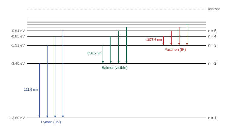
Each final level defines a series of lines. Transitions down to \(n = 1\) form the Lyman series, all in the ultraviolet, discovered by Theodore Lyman at Harvard between 1906 and 1914. Transitions to \(n = 2\) form the Balmer series, whose first four lines are visible. Transitions to \(n = 3\), 4 and 5 form the Paschen, Brackett and Pfund series in the infrared. Each series crowds toward a series limit, the wavelength for a jump from the edge of ionization.

# Hydrogen spectral series from E_n = -13.6057 eV / n^2, with the reduced-mass correction
Ry_eV = 13.605693        # Rydberg energy for infinite nuclear mass
me_over_mp = 1 / 1836.15267
Ry_H = Ry_eV / (1 + me_over_mp)
hc = 1239.84198           # eV nm
series = {1: "Lyman", 2: "Balmer", 3: "Paschen", 4: "Brackett"}
for n1, name in series.items():
    lines = []
    for n2 in range(n1 + 1, n1 + 5):
        dE = Ry_H * (1 / n1**2 - 1 / n2**2)
        lines.append(f"{hc / dE:8.1f}")
    limit = hc / (Ry_H / n1**2)
    print(f"{name:9s} (to n = {n1}): first lines {', '.join(lines)} nm; limit {limit:7.1f} nm")
print(f"ionization energy of hydrogen: {Ry_H:.4f} eV")
for Z, ion in ((2, "He+"), (3, "Li2+")):
    print(f"{ion}: ground state {-Ry_eV * Z**2:7.2f} eV; the n = 4 -> 3 line at {hc / (Ry_eV * Z**2 * (1/9 - 1/16)):.1f} nm")
# the 21 cm line: hyperfine splitting of the ground state
f21 = 1420.405751768e6
print(f"hyperfine line: {f21 / 1e6:.3f} MHz, wavelength {2.99792458e8 / f21 * 100:.2f} cm, photon energy {4.135667696e-15 * f21 * 1e6:.2f} micro eV")

Lyman     (to n = 1): first lines    121.6,    102.6,     97.3,     95.0 nm; limit    91.2 nm
Balmer    (to n = 2): first lines    656.5,    486.3,    434.2,    410.3 nm; limit   364.7 nm
Paschen   (to n = 3): first lines   1875.6,   1282.2,   1094.1,   1005.2 nm; limit   820.6 nm
Brackett  (to n = 4): first lines   4052.3,   2625.9,   2166.1,   1945.1 nm; limit  1458.8 nm
ionization energy of hydrogen: 13.5983 eV
He+: ground state  -54.42 eV; the n = 4 -> 3 line at 468.7 nm
Li2+: ground state -122.45 eV; the n = 4 -> 3 line at 208.3 nm
hyperfine line: 1420.406 MHz, wavelength 21.11 cm, photon energy 5.87 micro eV

The computed wavelengths are vacuum values; the Balmer line \(H\alpha\) appears at 656.3 nm in air. The \(n = 4 \to 3\) line of ionized helium at 468.7 nm (468.6 nm in air) is one of the lines Bohr assigned. The last line of output is not in Bohr's model at all. The proton and electron each have a magnetic moment from their spin, lesson 10, and the ground state is split into two levels by their interaction. The transition between them emits radio waves at 1420 MHz, the famous 21 cm line. Predicted by Hendrik van de Hulst in 1944 and detected by Harold Ewen and Edward Purcell at Harvard in 1951, it lets radio astronomers map cold hydrogen throughout the Milky Way and in distant galaxies; the spiral arms of our galaxy were first traced with it.

Schrödinger's hydrogen atom

Bohr's model is wrong in detail. It gives the ground state an angular momentum of \(\hbar\), when it actually has none, and it fails completely for helium and every heavier atom. The Schrödinger equation in three dimensions, with the Coulomb potential \(U = -ke^2/r\), can be solved exactly by separating it in spherical coordinates. The solutions are labeled by three quantum numbers:

• The principal quantum number \(n = 1, 2, 3, \ldots\) sets the energy, \(E_n = -13.6\ \mathrm{eV}/n^2\), exactly as in Bohr's model.
• The orbital quantum number \(l = 0, 1, \ldots, n - 1\) sets the magnitude of the orbital angular momentum, \(L = \sqrt{l(l+1)}\,\hbar\). States with \(l = 0, 1, 2, 3\) are called s, p, d and f, letters inherited from nineteenth-century spectroscopy (sharp, principal, diffuse, fundamental).
• The magnetic quantum number \(m_l = -l, \ldots, +l\) sets the component of angular momentum along a chosen axis, \(L_z = m_l \hbar\).

For each \(n\) there are \(n^2\) combinations of \(l\) and \(m_l\), all with the same energy, a degeneracy special to the \(1/r\) potential. The angular momentum can never point exactly along the axis, because \(|m_l| \le l < \sqrt{l(l+1)}\); this is another face of the uncertainty principle. The ground state is \(1s\), with \(n = 1\), \(l = 0\), a spherical cloud with zero angular momentum.

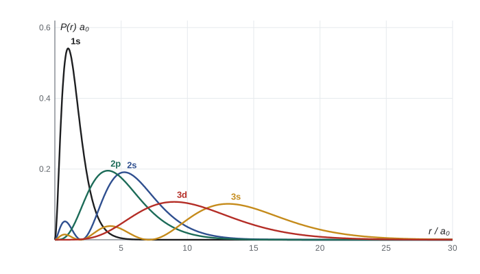
The probability of finding the electron between radii \(r\) and \(r + dr\) is the radial probability density \(P(r)\,dr = |R_{nl}(r)|^2 r^2\,dr\), where \(R_{nl}\) is the radial part of the wave function. For the ground state \(R_{10} \propto e^{-r/a_0}\), so \(P(r) \propto r^2 e^{-2r/a_0}\), which peaks exactly at \(r = a_0\). Bohr's orbit survives as the most probable radius of a smeared-out cloud. The excited states have \(n - l - 1\) radial nodes, spherical shells where the electron is never found.

import math
# radial wave functions of hydrogen in units of a0 (unnormalized), from the standard formulas
R = {
    "1s": lambda r: math.exp(-r),
    "2s": lambda r: (2 - r) * math.exp(-r / 2),
    "2p": lambda r: r * math.exp(-r / 2),
    "3s": lambda r: (27 - 18 * r + 2 * r * r) * math.exp(-r / 3),
    "3p": lambda r: r * (6 - r) * math.exp(-r / 3),
    "3d": lambda r: r * r * math.exp(-r / 3),
}
dr, rmax = 0.001, 60.0
rs = [(i + 0.5) * dr for i in range(int(rmax / dr))]
for name, f in R.items():
    P = [(f(r) * r) ** 2 for r in rs]
    norm = sum(P) * dr
    mean_r = sum(r * p for r, p in zip(rs, P)) * dr / norm
    peak = rs[max(range(len(P)), key=P.__getitem__)]
    nodes = sum(1 for a, b in zip(rs[:-1], rs[1:]) if f(a) * f(b) < 0)
    inside = sum(p for r, p in zip(rs, P) if r < 1.0) * dr / norm
    print(f"{name}: most probable r = {peak:5.2f} a0, mean r = {mean_r:6.2f} a0, radial nodes = {nodes},"
          f" probability inside a0 = {inside:.3f}")

1s: most probable r =  1.00 a0, mean r =   1.50 a0, radial nodes = 0, probability inside a0 = 0.323
2s: most probable r =  5.24 a0, mean r =   6.00 a0, radial nodes = 1, probability inside a0 = 0.034
2p: most probable r =  4.00 a0, mean r =   5.00 a0, radial nodes = 0, probability inside a0 = 0.004
3s: most probable r = 13.07 a0, mean r =  13.50 a0, radial nodes = 2, probability inside a0 = 0.010
3p: most probable r = 12.00 a0, mean r =  12.50 a0, radial nodes = 1, probability inside a0 = 0.001
3d: most probable r =  9.00 a0, mean r =  10.50 a0, radial nodes = 0, probability inside a0 = 0.000

The numerical integration confirms the analytic results. The \(1s\) state peaks at \(a_0\) with a mean radius of \(1.5\,a_0\), and the electron spends about 32% of its time inside the Bohr radius. The formula for the mean radius, \(\langle r \rangle = \tfrac12\big(3n^2 - l(l+1)\big) a_0\), shows that states with low \(l\) reach farther out on average but also penetrate closer to the nucleus. That penetration is crucial in many-electron atoms, lesson 10, where an inner \(s\) electron feels more of the nuclear charge than a \(p\) or \(d\) electron of the same \(n\).

Selection rules and the Zeeman effect

Not every pair of levels is connected by a spectral line. A photon carries one unit of angular momentum, so in the usual electric dipole transitions the orbital quantum number must change by one, \(\Delta l = \pm 1\), and \(m_l\) by 0 or \(\pm 1\). An electron in the \(2s\) state cannot jump to \(1s\) by emitting a single photon; it lives about a tenth of a second, very long by atomic standards, before decaying by emitting two photons at once. The \(2p\) state, in contrast, decays to \(1s\) in 1.6 ns, emitting the Lyman alpha line.

In a magnetic field the states with different \(m_l\) acquire slightly different energies, \(\Delta E = m_l \mu_B B\), with the Bohr magneton \(\mu_B = e\hbar/2m = 5.79 \times 10^{-5}\ \mathrm{eV/T}\). A spectral line splits into several components, the Zeeman effect, discovered by Pieter Zeeman in 1896. Astronomers use it to measure magnetic fields on the Sun: George Ellery Hale found in 1908 that sunspots have fields of a few tenths of a tesla. The splitting is small, about 0.03 nm for a visible line in a 1 T field, but easily measured with a good spectrograph.

Precise spectroscopy has kept testing the hydrogen atom. Spin and relativity split the levels into fine structure, explained by Dirac's equation in 1928, and in 1947 Willis Lamb and Robert Retherford found a further tiny shift between the \(2s\) and \(2p\) levels, about 4 millionths of an electronvolt, which led to quantum electrodynamics. Today the \(1s\)–\(2s\) transition frequency has been measured to 15 significant figures by Theodor Hänsch's group, and the comparison with theory determines the Rydberg constant and the size of the proton.