Matter waves: de Broglie, electron diffraction and the uncertainty principle

If light, long thought to be a wave, also behaves as a stream of particles, might electrons, long thought to be particles, also behave as waves? Louis de Broglie, a French aristocrat who had studied history before turning to physics, proposed exactly that in his doctoral thesis of 1924. His examiners were unsure what to make of it and sent a copy to Einstein, who replied that de Broglie had lifted a corner of the great veil. Within three years the waves had been seen in electron diffraction experiments in New York and Aberdeen, and Erwin Schrödinger had written down the equation they obey. This lesson introduces matter waves, the experiments that confirmed them, the way a wave packet represents a particle, and Werner Heisenberg's uncertainty principle.

The de Broglie wavelength

For a photon, \(p = h/\lambda\). De Broglie proposed that the same relation, read backwards, gives a wavelength to every particle with momentum \(p\):

For everyday objects this wavelength is absurdly small. A 0.145 kg baseball at 40 m/s has \(\lambda = 6.626 \times 10^{-34}/(0.145 \times 40) = 1.1 \times 10^{-34}\) m, a hundred billion billion times smaller than a proton. No slit or crystal could ever diffract it, which is why baseballs follow Newton's laws. For an electron the wavelength is comparable with the spacing of atoms in a crystal. An electron accelerated from rest through a potential difference \(V\) has \(p = \sqrt{2meV}\) (non-relativistically), so

At 100 V the wavelength is 0.123 nm, just right for diffraction by a crystal lattice. De Broglie also gave his waves a frequency through \(E = hf\), and he pointed out that the stable orbits of Bohr's hydrogen atom, lesson 9, are exactly those in which a whole number of wavelengths fits around the circumference, \(2\pi r = n\lambda\). That is equivalent to Bohr's rule that the angular momentum is a multiple of \(h/2\pi\), and it was the first physical explanation of why only certain orbits are allowed.

Electrons diffract

Clinton Davisson and Lester Germer at Bell Telephone Laboratories in New York were studying how electrons scatter from metal surfaces. In 1925 a vacuum accident oxidized their nickel target, and they heated it to clean it. The heating recrystallized the nickel into a few large crystals, and afterwards the scattered electrons came off in sharp beams at particular angles. By 1927 they had shown that 54 eV electrons gave a strong reflection at 50 degrees from the incident beam, precisely as expected for waves of wavelength 0.167 nm diffracted by rows of nickel atoms 0.215 nm apart. In the same year George Paget Thomson at Aberdeen fired faster electrons through thin metal foils and photographed diffraction rings like those of X-rays. Davisson and Thomson shared the 1937 Nobel Prize. There is a pleasing irony in the second award: G. P. Thomson's father, J. J. Thomson, had won the 1906 prize for showing that the electron is a particle.

The geometry of the Davisson–Germer experiment is that of a reflection grating. The surface atoms form rows spaced \(d\) apart; waves scattered from adjacent rows reinforce when the path difference \(d\sin\phi\) equals a whole number of wavelengths, where \(\phi\) is the angle from the incident direction for normal incidence. The program below computes the predicted angle and compares the de Broglie wavelength with the value from the lattice.

import math
h, me, e = 6.62607015e-34, 9.1093837e-31, 1.602176634e-19
def lam_electron(V):
    p = math.sqrt(2 * me * e * V)
    return h / p
d = 0.215e-9                     # spacing of surface rows of nickel atoms, m
V = 54.0
lam = lam_electron(V)
phi = math.degrees(math.asin(lam / d))
print(f"de Broglie wavelength at {V:.0f} V: {lam * 1e9:.4f} nm")
print(f"first-order peak at {phi:.1f} degrees from the incident beam (measured: 50)")
print(f"wavelength from the measured angle: {d * math.sin(math.radians(50)) * 1e9:.4f} nm")
print()
for name, m, v in (("baseball", 0.145, 40.0), ("dust grain 1 microgram", 1e-9, 0.01),
                   ("C60 molecule", 720 * 1.66054e-27, 220.0), ("thermal neutron", 1.675e-27, 2200.0)):
    print(f"{name:24s} lambda = {h / (m * v):.3e} m")
for V in (100, 10e3, 200e3):     # electron microscope voltages; relativistic momentum
    E0 = 0.51099895e6
    pc = math.sqrt((V + E0)**2 - E0**2)          # in eV
    lam_rel = 1239.84198 / pc                     # nm
    print(f"electron at {V / 1e3:6.1f} kV: lambda = {lam_rel * 1e3:8.3f} pm"
          f" (non-relativistic {lam_electron(V) * 1e12:8.3f} pm)")

de Broglie wavelength at 54 V: 0.1669 nm
first-order peak at 50.9 degrees from the incident beam (measured: 50)
wavelength from the measured angle: 0.1647 nm

baseball                 lambda = 1.142e-34 m
dust grain 1 microgram   lambda = 6.626e-23 m
C60 molecule             lambda = 2.519e-12 m
thermal neutron          lambda = 1.798e-10 m
electron at    0.1 kV: lambda =  122.637 pm (non-relativistic  122.643 pm)
electron at   10.0 kV: lambda =   12.205 pm (non-relativistic   12.264 pm)
electron at  200.0 kV: lambda =    2.508 pm (non-relativistic    2.742 pm)

The calculation reproduces the 50 degree peak within a degree. The table of wavelengths shows why we do not notice matter waves in daily life and why neutrons from a reactor, with wavelengths near 0.18 nm, are excellent for studying crystals. Canada's NRU reactor at Chalk River, which operated from 1957 to 2018, was a center of neutron scattering research, and Bertram Brockhouse shared the 1994 Nobel Prize for neutron spectroscopy methods he developed there. The last lines show that electrons in a 200 kV transmission electron microscope have a wavelength of 2.5 pm, small enough to resolve individual atoms, and that the relativistic correction is already more than 10% at that voltage.

The double slit, one electron at a time

The most striking demonstration of matter waves is the double-slit experiment. Claus Jönsson at Tübingen made electron double slits in 1961. In 1989 Akira Tonomura and colleagues at Hitachi used an electron biprism, a fine charged wire that splits an electron wave in two, with a beam so weak that only one electron at a time was in the apparatus. Each electron arrived as a single bright dot on the detector, at an apparently random place. After a few hundred electrons the dots looked scattered. After tens of thousands, they formed unmistakable interference fringes.

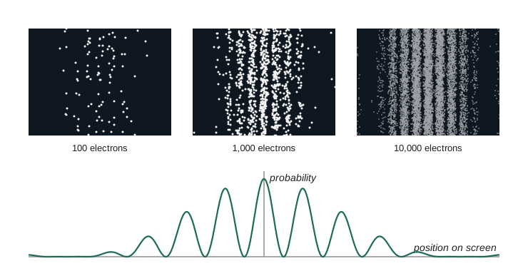
Each electron goes through the apparatus alone, yet the pattern shows interference between waves passing through both slits. If you put a detector at one slit to see which way each electron went, the fringes disappear, and you get the sum of two single-slit patterns. The wave that interferes is not a wave of many electrons; it is a wave of probability for each single electron. Max Born proposed this interpretation in 1926: the square of the wave's amplitude at a point gives the probability of finding the particle there. The program below simulates the arrival of individual electrons by sampling from the two-slit probability density.

import math, random
random.seed(1989)
lam, d, a, L = 50e-12, 1.0e-6, 0.2e-6, 1.0      # wavelength, slit separation, slit width, distance (m)
def density(x):
    s = x / L                                     # small-angle sine
    beta = math.pi * a * s / lam
    env = 1.0 if beta == 0 else (math.sin(beta) / beta) ** 2
    return env * math.cos(math.pi * d * s / lam) ** 2
xmax = 3 * lam * L / a                           # out to the third envelope zero
def sample():
    while True:                                   # rejection sampling
        x = random.uniform(-xmax, xmax)
        if random.random() < density(x):
            return x
fringe = lam * L / d
print(f"fringe spacing = {fringe * 1e6:.1f} micro m; envelope zero at {lam * L / a * 1e6:.1f} micro m")
for N in (100, 2000, 20000):
    xs = [sample() for _ in range(N)]
    bins = [0] * 12
    for x in xs:
        k = int((x + 3 * fringe + fringe / 4) // (fringe / 2))   # bins on bright and dark fringes
        if 0 <= k < 12:
            bins[k] += 1
    print(f"N = {N:6d}: bright/dark/bright... bins {bins}")

fringe spacing = 50.0 micro m; envelope zero at 250.0 micro m
N =    100: bright/dark/bright... bins [1, 1, 8, 3, 20, 2, 21, 3, 17, 2, 12, 3]
N =   2000: bright/dark/bright... bins [91, 23, 199, 61, 320, 82, 319, 73, 307, 58, 195, 28]
N =  20000: bright/dark/bright... bins [873, 347, 1940, 567, 2869, 710, 3436, 713, 2925, 577, 1838, 343]

The bins alternate between the centers of bright fringes and the centers of dark ones. With 100 electrons each bin holds only a handful of counts, and on a screen the dots would look almost random. With 20,000 the alternation is unmistakable: the central bright bin collects about 3,400 electrons and its dark neighbors about 700 each. The dark bins are not empty because each bin is half a fringe wide and catches the sides of the bright fringes. Interference is a statistical property of many single events, each governed by a probability wave. Interference has since been seen with neutrons, atoms and molecules: in 1999 Anton Zeilinger's group in Vienna diffracted buckminsterfullerene, C60, with 60 carbon atoms, and later experiments have used molecules of more than 2,000 atoms.

Wave packets

A wave of a single wavelength, \(\psi = A\cos(kx - \omega t)\) with \(k = 2\pi/\lambda\), extends forever and has the same amplitude everywhere. It describes a particle with a perfectly definite momentum \(p = \hbar k\), where \(\hbar = h/2\pi\), but no definite position at all. To describe a particle that is somewhere in particular, we add waves with a range of wavelengths. They reinforce in a small region and cancel elsewhere, forming a wave packet. PHYS-230 showed that a packet built from a spread \(\Delta k\) of wave numbers has a width \(\Delta x\) with \(\Delta x\,\Delta k \gtrsim 1\): narrow packets need many wavelengths, and a single wavelength needs infinite length. This is a property of all waves, from sound to radio, where it limits how short a pulse can be for a given bandwidth.

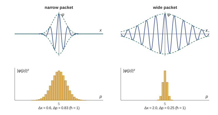
For matter waves, the packet moves at the group velocity \(d\omega/dk\). With \(E = \hbar\omega\) and \(p = \hbar k\), the group velocity is \(dE/dp\), which for a free particle with \(E = p^2/2m\) is \(p/m = v\), the particle's velocity. The phase velocity of the individual crests, \(\omega/k = v/2\), has no direct meaning. Because \(\omega\) is not proportional to \(k\), matter waves are dispersive, and a packet spreads as it moves, the narrower it starts the faster it spreads.

The uncertainty principle

Combining \(\Delta x\,\Delta k \gtrsim 1\) with \(p = \hbar k\) gives a limit on how precisely a particle's position and momentum can both be specified. The exact statement, proved by Earle Kennard in 1927 from the mathematics of Fourier transforms, uses standard deviations:

The equality holds only for a Gaussian packet. Heisenberg introduced the principle in 1927 with a thought experiment, the gamma-ray microscope: to locate an electron precisely you must scatter short-wavelength light from it, and each scattered photon gives it an unpredictable kick, as in Compton scattering. But the principle is not about clumsy measurements. It is a statement that a particle does not have a precise position and a precise momentum at the same time, because it is described by a wave. The program below builds Gaussian packets of different widths, computes their momentum distributions by direct numerical Fourier transform, and checks that the product of the spreads is \(\hbar/2\).

import math, cmath
def spreads(sigma, N=1201, span=12.0, kmax=None):
    # psi(x) = exp(-x^2 / (4 sigma^2)) exp(i k0 x); units with hbar = 1, so p = k
    k0 = 5.0
    dx = span * sigma / (N - 1)
    xs = [-span * sigma / 2 + i * dx for i in range(N)]
    psi = [math.exp(-x * x / (4 * sigma * sigma)) * cmath.exp(1j * k0 * x) for x in xs]
    norm = sum(abs(p)**2 for p in psi) * dx
    mx = sum(x * abs(p)**2 for x, p in zip(xs, psi)) * dx / norm
    sx = math.sqrt(sum((x - mx)**2 * abs(p)**2 for x, p in zip(xs, psi)) * dx / norm)
    # momentum amplitude phi(k) by direct summation
    kmax = k0 + 6 / sigma
    ks = [k0 - 6 / sigma + j * (12 / sigma) / 200 for j in range(201)]
    phik = [abs(sum(p * cmath.exp(-1j * k * x) for x, p in zip(xs, psi)) * dx)**2 for k in ks]
    dk = ks[1] - ks[0]
    nk = sum(phik) * dk
    mk = sum(k * w for k, w in zip(ks, phik)) * dk / nk
    sk = math.sqrt(sum((k - mk)**2 * w for k, w in zip(ks, phik)) * dk / nk)
    return sx, sk, mk
for sigma in (0.5, 1.0, 2.0, 4.0):
    sx, sp, mean_p = spreads(sigma)
    print(f"sigma = {sigma:3.1f}: dx = {sx:.4f}, dp = {sp:.4f}, dx*dp = {sx * sp:.4f} (hbar/2 = 0.5), <p> = {mean_p:.3f}")
hbar, me = 1.054571817e-34, 9.1093837e-31
dx_atom = 0.05e-9
dp = hbar / (2 * dx_atom)
print(f"electron confined to 0.05 nm: dp >= {dp:.2e} kg m/s, kinetic energy ~ {dp**2 / (2 * me) / 1.602e-19:.1f} eV")

sigma = 0.5: dx = 0.5000, dp = 1.0000, dx*dp = 0.5000 (hbar/2 = 0.5), <p> = 5.000
sigma = 1.0: dx = 1.0000, dp = 0.5000, dx*dp = 0.5000 (hbar/2 = 0.5), <p> = 5.000
sigma = 2.0: dx = 2.0000, dp = 0.2500, dx*dp = 0.5000 (hbar/2 = 0.5), <p> = 5.000
sigma = 4.0: dx = 4.0000, dp = 0.1250, dx*dp = 0.5000 (hbar/2 = 0.5), <p> = 5.000
electron confined to 0.05 nm: dp >= 1.05e-24 kg m/s, kinetic energy ~ 3.8 eV

Every Gaussian packet gives a product of exactly 0.5 in units of \(\hbar\), whatever its width: making it narrower in position makes it wider in momentum. The last line shows why atoms have the size they do. An electron confined to a region 0.05 nm across must have a momentum spread that corresponds to a kinetic energy of several electronvolts, comparable with atomic binding energies. Squeezing the electron closer to the nucleus would lower its potential energy but raise its kinetic energy more, so there is a minimum total energy at a radius near the Bohr radius. The uncertainty principle is what keeps atoms from collapsing, the problem that defeated classical physics in lesson 1.

There is a similar relation between energy and time, \(\Delta E\,\Delta t \gtrsim \hbar/2\), where \(\Delta t\) is the time over which a system changes appreciably. An excited atomic state that lives for 10 ns has an energy width of about \(10^{-7}\) eV, which shows up as the natural width of its spectral line. Very short-lived particles, such as the Z boson with a lifetime of \(3 \times 10^{-25}\) s, have widths of a few GeV that can be measured directly in collider experiments.