Photons: the photoelectric effect, Compton scattering and pair production

In March 1905, three months before his paper on relativity, Einstein submitted a paper on the production and transformation of light that he himself called very revolutionary. He proposed that light behaves, in some experiments, as if it consisted of independent packets of energy \(hf\), which he called light quanta and which we now call photons. The idea explained the photoelectric effect at once, but it met strong resistance for nearly twenty years, because the wave theory of light had overwhelming support from interference and diffraction. Two experiments changed minds: Robert Millikan's careful measurements of the photoelectric effect, completed in 1916, and Arthur Compton's discovery in 1923 that X-rays scatter from electrons like billiard balls. This lesson covers both, and then the creation and annihilation of matter by photons, which underlies PET scanning.

The photoelectric effect

Light shining on a clean metal surface in vacuum ejects electrons, called photoelectrons. In a typical apparatus the metal is one electrode of a phototube, and a variable voltage between the electrodes either helps or opposes the electrons on their way to the collector. When the collector is made negative enough, even the fastest electrons are turned back and the current stops. The voltage at which this happens is the stopping potential \(V_s\), and \(eV_s\) is the maximum kinetic energy of the photoelectrons.

Experiments by Lenard and others established four facts. The photocurrent is proportional to the intensity of the light. The stopping potential, and so the maximum kinetic energy, does not depend on intensity. The stopping potential increases linearly with the frequency of the light. And for each metal there is a threshold frequency below which no electrons are emitted at all, however intense the light. Emission also begins without measurable delay, within a nanosecond, even at very low intensity, when a classical calculation suggests that an atom would need minutes to absorb enough energy from a feeble wave.

Einstein's explanation was that each photoelectron is ejected by a single photon. The photon gives up all its energy \(hf\); part of it, at least the work function \(\phi\) of the metal, is needed to free the electron from the surface, and the rest becomes kinetic energy:

This accounts for every observation. Brighter light means more photons and therefore more electrons, but each photon has the same energy. A higher frequency means more energetic photons. The threshold is \(f_0 = \phi/h\). And there is no delay because the energy arrives in a single packet. Work functions are a few electronvolts: about 2.1 eV for cesium, 2.3 eV for sodium, 4.3 eV for zinc and 5.1 eV for platinum.

Millikan's measurement of h

Millikan set out to disprove Einstein's equation. Working at the University of Chicago, he built an apparatus in which fresh surfaces of sodium, potassium and lithium were cut with a knife operated by an electromagnet inside the vacuum, so that the surfaces were free of oxide. After ten years of work he published in 1916 a straight line of stopping potential against frequency whose slope, \(h/e\), gave \(h = 6.57 \times 10^{-34}\ \mathrm{J\,s}\), within 0.5% of Planck's value from blackbody radiation. He confirmed the equation exactly, while still doubting the photon picture behind it. Einstein received the 1921 Nobel Prize for the law of the photoelectric effect, and Millikan the 1923 prize partly for this work.

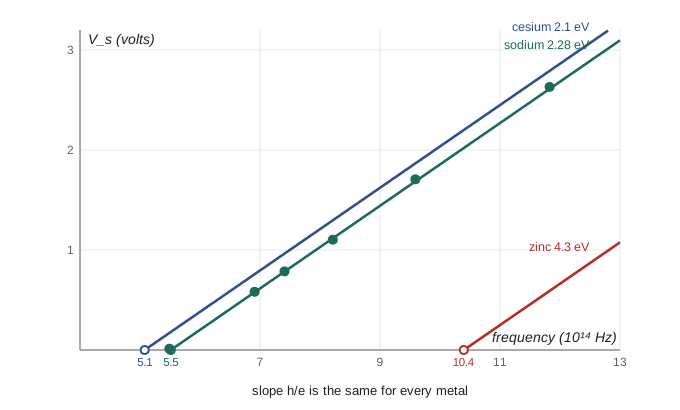
The program below plays the part of Millikan's analysis. It generates stopping potentials for sodium at the wavelengths of the mercury lines that Millikan used, adds measurement noise from a fixed random seed, and fits a straight line by least squares. The slope gives \(h/e\) and the intercept gives the work function.

import random
random.seed(1902)
h_true, e, c = 6.62607015e-34, 1.602176634e-19, 2.99792458e8
phi_true = 2.28                                  # sodium work function, eV
wavelengths_nm = [546.1, 433.9, 404.7, 365.0, 312.6, 253.5]   # mercury lines
f = [c / (w * 1e-9) for w in wavelengths_nm]
V = [h_true * fi / e - phi_true + random.gauss(0, 0.02) for fi in f]
n = len(f)
fm, Vm = sum(f) / n, sum(V) / n
Sxx = sum((x - fm)**2 for x in f)
slope = sum((x - fm) * (y - Vm) for x, y in zip(f, V)) / Sxx
icept = Vm - slope * fm
res = [y - (slope * x + icept) for x, y in zip(f, V)]
s2 = sum(r * r for r in res) / (n - 2)
s_slope = (s2 / Sxx) ** 0.5
for w, fi, Vi in zip(wavelengths_nm, f, V):
    print(f"{w:6.1f} nm  f = {fi / 1e14:6.3f} x 1e14 Hz  V_s = {Vi:6.3f} V")
print(f"slope h/e = {slope:.4e} +/- {s_slope:.1e} V s")
print(f"h = {slope * e:.4e} J s  (true {h_true:.4e})")
print(f"work function = {-icept:.3f} eV, threshold f0 = {-icept / slope / 1e14:.3f} x 1e14 Hz,"
      f" threshold wavelength {c / (-icept / slope) * 1e9:.0f} nm")

 546.1 nm  f =  5.490 x 1e14 Hz  V_s =  0.013 V
 433.9 nm  f =  6.909 x 1e14 Hz  V_s =  0.582 V
 404.7 nm  f =  7.408 x 1e14 Hz  V_s =  0.786 V
 365.0 nm  f =  8.213 x 1e14 Hz  V_s =  1.103 V
 312.6 nm  f =  9.590 x 1e14 Hz  V_s =  1.707 V
 253.5 nm  f = 11.826 x 1e14 Hz  V_s =  2.631 V
slope h/e = 4.1467e-15 +/- 3.1e-17 V s
h = 6.6437e-34 J s  (true 6.6261e-34)
work function = 2.280 eV, threshold f0 = 5.497 x 1e14 Hz, threshold wavelength 545 nm

Six points with 20 millivolt errors give \(h\) to better than 1%. The 546 nm green line is barely above the threshold for sodium, so its electrons have only a few hundredths of an electronvolt of energy; red light, at wavelengths longer than the 545 nm threshold, would eject none at all. The same physics operates in every photomultiplier tube, the detectors that count single photons in neutrino observatories such as SNOLAB near Sudbury and Super-Kamiokande in Japan, and in the image sensors of early television cameras.

Photon energy and momentum

A photon of frequency \(f\) and wavelength \(\lambda = c/f\) has energy and momentum

The combination \(hc = 1240\ \mathrm{eV\,nm}\) is worth memorizing: a 620 nm red photon has 2.0 eV, a 124 nm ultraviolet photon 10 eV, a 0.124 nm X-ray 10 keV. Photons from an FM radio station at 100 MHz have only \(4 \times 10^{-7}\) eV, so a 50 kW transmitter emits about \(8 \times 10^{29}\) photons per second, and the graininess of the wave is utterly undetectable. The momentum of light is real: it exerts radiation pressure, which pushes the tails of comets away from the Sun and drove the Japanese solar sail IKAROS across the solar system in 2010.

Compton scattering

In 1923 Arthur Compton at Washington University in St. Louis directed X-rays from a molybdenum target, wavelength 0.0709 nm, onto a block of graphite and measured the wavelength of the scattered X-rays with a crystal spectrometer. At each scattering angle he found two peaks: one at the original wavelength, and one shifted to a longer wavelength by an amount that grew with the angle. A classical wave scattered by a free electron makes the electron oscillate at the wave's frequency and re-radiate at the same frequency, so there should be no shift at all.

Compton explained the shift by treating the X-ray as a photon that collides elastically with a free electron at rest. Conservation of energy and momentum, with the relativistic expressions of lesson 4, does the rest. Let the incoming photon have momentum \(p = h/\lambda\), the scattered photon \(p' = h/\lambda'\) at angle \(\theta\), and the recoiling electron momentum \(\mathbf{p}_e\). Momentum conservation gives \(\mathbf{p}_e = \mathbf{p} - \mathbf{p}'\), so

Energy conservation gives \(pc + mc^2 = p'c + E_e\), with \(E_e^2 = (p_e c)^2 + (mc^2)^2\). Squaring \(E_e = (p - p')c + mc^2\) and substituting for \(p_e^2\):

The \(p^2\), \(p'^2\) and \(m^2c^4\) terms cancel, leaving \(-2pp' + 2(p - p') mc = -2pp' \cos\theta\), or \((p - p') mc = pp'(1 - \cos\theta)\). Dividing by \(pp'mc\) and using \(1/p = \lambda/h\):

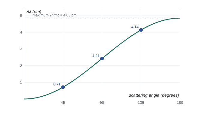
The constant \(h/mc = 2.426 \times 10^{-12}\) m is the Compton wavelength of the electron. The shift does not depend on the incident wavelength, so it is a large fraction of the wavelength only for X-rays and gamma rays; for visible light it is a millionth of the wavelength and unobservable. The unshifted peak comes from photons scattering off tightly bound inner electrons, for which the whole atom recoils and \(m\) is effectively thousands of times larger.

import math
h, me, c, e = 6.62607015e-34, 9.1093837e-31, 2.99792458e8, 1.602176634e-19
lam_C = h / (me * c)
print(f"Compton wavelength of the electron: {lam_C * 1e12:.4f} pm")
lam0 = 70.9e-12          # Mo K-alpha X-rays, as in Compton's experiment
E0 = h * c / lam0 / e
print(f"incident X-ray: {lam0 * 1e12:.1f} pm, {E0 / 1000:.2f} keV")
for deg in (0, 45, 90, 135, 180):
    th = math.radians(deg)
    lam1 = lam0 + lam_C * (1 - math.cos(th))
    E1 = h * c / lam1 / e
    print(f"theta = {deg:3d} deg: scattered {lam1 * 1e12:7.3f} pm, photon {E1 / 1000:6.3f} keV,"
          f" electron gets {(E0 - E1):6.1f} eV")
# a 662 keV gamma ray (from Cs-137) backscattered: the 'Compton edge' seen in detectors
Eg = 662e3; m = 511e3
E_back = Eg / (1 + 2 * Eg / m)
print(f"662 keV gamma backscattered: photon {E_back / 1000:.0f} keV, electron {(Eg - E_back) / 1000:.0f} keV")

Compton wavelength of the electron: 2.4263 pm
incident X-ray: 70.9 pm, 17.49 keV
theta =   0 deg: scattered  70.900 pm, photon 17.487 keV, electron gets    0.0 eV
theta =  45 deg: scattered  71.611 pm, photon 17.314 keV, electron gets  173.5 eV
theta =  90 deg: scattered  73.326 pm, photon 16.909 keV, electron gets  578.6 eV
theta = 135 deg: scattered  75.042 pm, photon 16.522 keV, electron gets  965.2 eV
theta = 180 deg: scattered  75.753 pm, photon 16.367 keV, electron gets 1120.2 eV
662 keV gamma backscattered: photon 184 keV, electron 478 keV

For Compton's X-rays the electron receives only a few hundred electronvolts. For gamma rays the share is large: a 662 keV photon from a Cs-137 calibration source can transfer up to 478 keV to an electron, which produces the sharp Compton edge seen in the spectrum of every gamma-ray detector. Compton scattering is also the main way X-rays and gamma rays deposit energy in soft tissue at the energies used in radiation therapy, and the reason that a CT scanner's image depends mostly on electron density.

Pair production and annihilation

A photon with energy above \(2mc^2 = 1.022\) MeV can turn into an electron and a positron, the electron's antiparticle, predicted by Paul Dirac in 1928 and discovered by Carl Anderson in cosmic rays in 1932. The conversion needs a nearby nucleus to absorb some momentum: a single photon in empty space cannot become a pair, because in the pair's center-of-momentum frame the total momentum is zero while the photon's is not. Above about 10 MeV, pair production is the dominant way that high-energy photons interact with matter.

The reverse process is annihilation. A positron slows down in matter and meets an electron, and the two disappear, producing almost always two photons of 511 keV each, emitted back to back so that their total momentum is zero. Positron emission tomography uses exactly this. A patient receives a sugar molecule labeled with fluorine-18, which decays by emitting a positron. The positron travels about a millimeter, annihilates, and the two 511 keV photons fly off in opposite directions to a ring of detectors. Each coincident pair defines a line through the point of annihilation, and millions of such lines are combined into a three-dimensional image of where the sugar is being used, which reveals active tumors and brain regions. Lesson 12 returns to PET.

Wave or particle?

Light diffracts and interferes like a wave, PHYS-230 showed in detail, and it transfers energy and momentum in lumps like a particle. Neither picture alone is complete. In 1909 Geoffrey Taylor photographed the diffraction pattern of a needle with light so dim that only about one photon at a time was in the apparatus; after three months of exposure the full pattern appeared. Each photon arrives at one point, but the probability of arriving at each point follows the wave pattern. This combination, quantized arrival and wave-like probability, is the core of quantum mechanics, and lesson 7 shows that electrons and all other particles behave the same way.