
NUC-330 · Lesson 8 of 12 · 22 min
Core thermal design limits
Rohan's group delivers its results to the utility as margins: how far the hottest fuel is from each limit, and what eats into that distance. For TVA's uprate study, the question is how much of a modest power increase the existing margins can absorb, after every uncertainty has been accounted for. "An uprate does not change the limits," Rohan says. "It moves the operating point toward them. Our job is to show exactly how far it can move."
What the limits protect
Thermal design limits exist to keep the fuel intact and the coolant system able to cool it, in normal operation and in anticipated operational occurrences, the transients expected to happen once or more in a plant's life, such as a loss of one pump or an inadvertent control rod withdrawal. Each limit protects against a particular failure mechanism.
| Limit | Protects against | Typical form |
|---|---|---|
| Peak linear heat rate | fuel center melting, excessive fission gas release, loss-of-coolant stored energy | maximum q' in kW/m, sometimes burnup-dependent |
| Minimum DNBR | sheath overheating after DNB in PWRs | minimum DNBR above a statistical design limit |
| Minimum critical power ratio | dryout in BWR bundles | MCPR above the safety limit plus an operating margin |
| Channel and bundle power limits (CANDU) | dryout, fuel overpower | maximum channel and bundle powers, regional overpower protection |
| Sheath temperature and strain | corrosion, creep, pellet-cladding interaction | limits on power increases and ramp rates |
| Coolant conditions | boiling where it is not intended, pump cavitation | limits on inlet temperature, pressure and flow |
Hot channel factors
Lesson 1 introduced the nuclear peaking factors, which describe the calculated power distribution. Real fuel also differs slightly from its drawings. Pellets vary in density and enrichment within tolerances, rods vary in diameter, the pitch between rods varies, and pellets sit off-center in the sheath. Each deviation can make some local heat flux, enthalpy rise or temperature slightly worse than the nominal calculation predicts. These are handled with engineering hot channel factors.
The nuclear factor \(F_q^{N}\) comes from the physics calculation, measured and confirmed in operation, with its own measurement uncertainty. The engineering factor \(F_q^{E}\) combines the manufacturing deviations. Historically, all factors were multiplied together, as if every deviation were at its worst at the same place at the same time. That is conservative, often very conservative.
Deterministic versus statistical combination
Statistical methods recognize that independent random deviations rarely all reach their extremes together. If each engineering factor is written as \(1 + \delta_i\), where \(\delta_i\) is a deviation at the same confidence level, a root-sum-square combination gives
which is smaller than the product \(\prod (1 + \delta_i)\). Modern design methods go further and combine uncertainties in power, flow, pressure, inlet temperature, correlation and manufacturing statistically, often by Monte Carlo propagation, to set a single statistically based design limit. Regulators accept these methods when the input uncertainties are well characterized and independent, and when the method has been reviewed.
Worked problem
Deterministic and statistical engineering factors
Three independent engineering deviations on local heat flux are 2 percent (pellet density and enrichment), 1.5 percent (rod diameter and pitch) and 1 percent (eccentricity). With a nuclear factor of 2.30 and an average linear heat rate of 17.8 kW/m, find the peak linear heat rate with the factors multiplied and with root-sum-square combination.
Show solution
- Product: \(1.02 \times 1.015 \times 1.01 = 1.046\); peak \(= 17.8 \times 2.30 \times 1.046 = 42.8\) kW/m.
- Root-sum-square: \(1 + \sqrt{0.02^2 + 0.015^2 + 0.01^2} = 1.027\); peak \(= 17.8 \times 2.30 \times 1.027 = 42.0\) kW/m.
Answer: 42.8 kW/m deterministically and 42.0 kW/m statistically. The difference, about 2 percent, is margin the plant can use without changing any physical limit.
The margin stack
Analysts often explain margin as a stack. At the bottom is the physical phenomenon, such as the true CHF. Above it is the safety limit, set with allowance for correlation uncertainty, for example the 95/95 DNBR limit. Above that is the analysis value, which includes allowances for instrument uncertainties, transient overshoot and modeling assumptions in the safety analysis. Above that again is the operating point, the predicted or measured value in normal operation. The gap between operating point and analysis value is operating margin; the gap between analysis value and safety limit is analytical margin; and the gap between the safety limit and the real phenomenon is the confidence built into the limit itself.
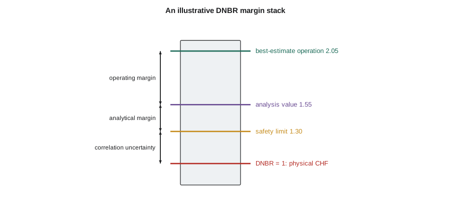
An uprate, a fuel design change, an instrument change or an aging mechanism moves one or more of these levels. Good margin management shows each move explicitly, so that the plant's owner and the regulator can see what is being used up and why. Rohan insists that every result his group sends out includes such a table.
# Hot-channel factors and thermal margins: deterministic product vs statistical combination.
import math
nuclear = {'F_q (local peaking)': 2.30, 'F_dH (enthalpy rise)': 1.55}
engineering = {'pellet density and enrichment': 1.02, 'rod diameter and pitch': 1.015, 'clad eccentricity': 1.01}
F_E = math.prod(engineering.values())
print(f"engineering factor, product = {F_E:.3f}")
# Statistical combination: treat each as a 2-sigma bound on a normal deviation
dev = [v - 1 for v in engineering.values()]
F_stat = 1 + math.sqrt(sum(d * d for d in dev))
print(f"engineering factor, root-sum-square = {F_stat:.3f}")
q_avg = 17.8   # kW/m
for name, F in (('deterministic', nuclear['F_q (local peaking)'] * F_E), ('statistical', nuclear['F_q (local peaking)'] * F_stat)):
    print(f"{name:13s}: peak linear heat rate = {q_avg*F:5.1f} kW/m")
# Margin stack for a minimum DNBR limit (illustrative numbers)
limit, analysis, measured = 1.30, 1.55, 2.05
print(f"DNBR: safety limit {limit}, analysis value {analysis}, best estimate {measured}")
print(f"  analytical margin {100*(analysis/limit-1):4.1f} %, operating margin {100*(measured/analysis-1):4.1f} %")
# CANDU aging: diametral creep lets coolant bypass the bundle, lowering critical channel power
for creep in (0.0, 2.0, 4.0, 5.1):
    ccp = 8.3 * (1 - 0.018 * creep)        # illustrative 1.8 % CCP loss per % diametral creep
print(f"pressure tube creep {creep:3.1f} % -> critical channel power ~ {ccp:4.2f} MW")engineering factor, product = 1.046 engineering factor, root-sum-square = 1.027 deterministic: peak linear heat rate = 42.8 kW/m statistical : peak linear heat rate = 42.0 kW/m DNBR: safety limit 1.3, analysis value 1.55, best estimate 2.05 analytical margin 19.2 %, operating margin 32.3 % pressure tube creep 0.0 % -> critical channel power ~ 8.30 MW pressure tube creep 2.0 % -> critical channel power ~ 8.00 MW pressure tube creep 4.0 % -> critical channel power ~ 7.70 MW pressure tube creep 5.1 % -> critical channel power ~ 7.54 MW
Limits in operation
In a PWR, thermal limits are enforced in operation by a combination of measurements, technical specification limits and reactor protection. Core power distribution is monitored with in-core detectors and ex-core detectors; limits on axial flux difference and rod insertion keep the power shape within the envelope assumed in the analyzes. The reactor protection system has trips designed to protect DNBR, such as the overtemperature delta-T trip, which compares the measured loop temperature difference, a measure of power, with a setpoint that falls as coolant temperature rises and pressure falls. A separate overpower delta-T trip protects the linear heat rate limit. A power uprate requires the setpoints to be recalculated with the new conditions.
Aging and margin
Margins change through a plant's life. Fuel is redesigned, operating practices change, and components age. Some examples:
| Change | Effect on thermal margin | Typical response |
|---|---|---|
| Steam generator fouling or tube plugging | higher primary coolant temperatures for the same power, less DNBR or dryout margin | cleaning, lower power, adjusted setpoints |
| Pressure tube diametral creep (CANDU) | more bypass flow around bundles, lower critical channel power | lower ROP setpoints, operational adjustments, refurbishment |
| Higher fuel burnup | lower UO₂ conductivity and gap changes, different stored energy | burnup-dependent linear heat rate limits |
| New fuel designs | often higher CHF from improved grids or bundles | credited after full-scale tests |
| Instrument replacement | changed uncertainties | recalculated allowances |
For the uprate, Rohan's simple model starts with the margin table and asks how each entry changes with power. Linear heat rate rises in proportion to power. DNBR falls faster than power, because higher power also raises the coolant temperature and lowers CHF. He finds that a few percent of uprate is available after the instrument uncertainty improvements, which the plant has already made, are credited.
Limits during transients
Anticipated transients must also meet the thermal limits. A loss of flow, for example from a pump trip, lowers DNBR quickly as the flow coasts down while power drops only after the reactor trips. An uncontrolled withdrawal of a control rod bank raises local power. A drop in feedwater temperature raises reactivity in a BWR and power in the core. Safety analyzes calculate the minimum DNBR or minimum critical power ratio reached during each transient, with conservative assumptions, and show that it stays above the limit, which is why the analysis value in the margin stack sits above the safety limit. Lesson 11 returns to these transients and to accidents where the limits may be exceeded briefly but other acceptance criteria apply.
Hana's draft report for the week has one table with six rows and three columns: limit, analysis value, operating value. "That," Rohan says, tapping the table, "is what the plant manager reads. Everything else is how we got there."
Uncertainty sources in a thermal limit
A useful exercise is to list everything uncertain in a minimum DNBR calculation and decide how each is handled. The list is long, and it explains why thermal design is as much statistics as heat transfer.
| Source | Typical size (one standard deviation or bound) | How it is handled |
|---|---|---|
| Core power measurement | about 0.5 to 2 percent | calorimetric accuracy; better instruments allow uprates |
| Coolant flow | about 1 to 3 percent | measured and bounded; low-flow assumption in analysis |
| Pressure and inlet temperature | a few tenths of a megapascal and a kelvin or two | instrument uncertainty |
| Nuclear peaking factors | a few percent | measured with in-core detectors, with uncertainty allowance |
| Engineering tolerances | one to two percent each | engineering hot channel factors |
| CHF correlation | about 5 to 10 percent scatter | statistical design limit |
| Subchannel code and mixing | a few percent | benchmarking against tests |
Some of these are random and independent, such as pellet density in different rods; some are systematic and affect every channel the same way, such as a bias in the core power measurement. Statistical methods treat random uncertainties by combination and systematic ones by bounding. A common error in student work is to combine systematic uncertainties by root-sum-square as if they were random; another is to count the same uncertainty twice, once in an input and again in a limit. Rohan's group keeps a single uncertainty register for each analysis, with every item tagged as random or systematic and as already included or not.
Power uprates in practice
Power uprates fall into three broad classes. A measurement uncertainty recapture uprate, typically up to about 1.7 percent, uses more accurate feedwater flow instruments to reduce the power measurement allowance; the physical margins are unchanged, but less of them is reserved for measurement error. Stretch uprates of a few percent use existing margins in the design with little or no equipment change. Extended uprates of up to about 20 percent need major equipment changes such as high-pressure turbine replacement, larger pumps or new steam generators, and usually new fuel designs with higher CHF. Each class needs the thermal limits to be shown to remain satisfied, along with many other analyzes outside this course, such as structural and containment analyzes.
CANDU stations rarely seek uprates in the same way, because their channel powers are already limited by dryout margin and their trip setpoints, and the main concern through life is preserving margin as pressure tubes age.
Worked problem
Margin used by a small uprate
A PWR has a minimum DNBR analysis value of 1.55 against a safety limit of 1.30. Sensitivity studies show the minimum DNBR falls by about 1.3 percent for each 1 percent increase in power. How large an uprate leaves at least 5 percent analytical margin?
Show solution
- Required analysis value \(= 1.30 \times 1.05 = 1.365\).
- Allowed reduction \(= 1 - 1.365/1.55 = 11.9\) percent of DNBR.
- Power increase \(\approx 11.9 / 1.3 \approx 9\) percent, before any other limits are checked.
Answer: About 9 percent from DNBR alone. In practice, other limits, including linear heat rate, loss-of-coolant results and equipment capacities, usually limit an uprate before DNBR does.
Summary and key terms
- Core thermal limits protect against fuel melting, DNB, dryout, sheath damage and unwanted coolant conditions.
- Hot channel factors combine nuclear peaking with engineering deviations from manufacturing tolerances.
- Statistical combination of independent uncertainties gives less conservative but defensible factors than multiplication.
- Margins are presented as a stack: physical phenomenon, safety limit, analysis value and operating point.
- Limits are enforced in operation by power distribution monitoring, technical specifications and protective trips.
- Aging, fouling, burnup and design changes move margins and must be tracked through plant life.
- Hot channel factor
- A factor relating the hottest local value to the nominal or average value.
- Engineering factor
- A hot channel factor for deviations from nominal dimensions and composition.
- Root-sum-square
- Combination of independent deviations by the square root of the sum of their squares.
- Safety limit
- A limit on a process variable, set with uncertainty allowance, that must not be exceeded.
- Operating margin
- The difference between the operating value and the analysis value of a limited quantity.
- Regional overpower protection
- CANDU trip logic based on in-core detectors to prevent fuel dryout.
Practice problems
Work each problem on paper first, then reveal the answer to check.
Three independent deviations of 3, 2 and 1 percent: compare product and root-sum-square factors.
Show answer
Product 1.061; root-sum-square 1.037.
Why is multiplying all hot channel factors conservative?
Show answer
It assumes every deviation is at its worst at the same place and time, which is very unlikely.
If the DNBR safety limit is 1.30 and the analysis value 1.52, what is the analytical margin?
Show answer
About 17 percent.
Why does DNBR fall faster than power rises in an uprate?
Show answer
Higher power raises the heat flux and also raises coolant temperature and quality, lowering CHF.
How does pressure tube creep reduce CANDU margin?
Show answer
It lets more coolant bypass the bundle, lowering flow past the hottest elements and the critical channel power.
Lesson quiz · 5 questions
Score 60% or more to complete this lesson.
Create a free account to save your progress, take quizzes and earn a certificate.