Forecasting and sales and operations planning

Before the eighth session, Dr. Raman asks the cohort to find out how many numbers Cedarline uses for next year's sales. The answer arrives by email from the teams the following week: at least four. The merchandising team buys to a sales plan set by the chief executive, 7 percent above last year. Finance's budget assumes 4 percent growth, because it remembers that last year's plan was missed. The distribution center plans staff and space on a third number, last year's volumes plus whatever the warehouse manager hears in meetings. And the website team forecasts its own traffic with a statistical model that nobody outside the team has seen. Dr. Raman says this is common and costly. A company with four forecasts effectively has none, because each function acts on a different view of the future and the gaps are paid for in inventory, overtime and lost sales.

What forecasts are for

A forecast is an estimate of future demand that supports a decision: how much fabric to buy, how many agents to schedule, how big to build a warehouse. Three principles guide its use. First, forecasts are always wrong, so a good forecast comes with an estimate of its likely error, which plans then use to set buffers. Second, aggregate forecasts are more accurate than detailed ones: total jacket sales for a season are easier to forecast than sales of medium blue jackets in one store in one week, because errors at the detailed level partly cancel when added up. Third, forecasts for the near future are more accurate than for the distant future. Each principle has an operational consequence. Firms that can postpone detailed decisions, commit at an aggregate level and shorten lead times face smaller forecast errors, which is the logic of the supply chain designs in lessons 10 to 12.

Forecasting methods fall into two families. Qualitative methods rely on judgment: the views of salespeople, executives or experts, customer surveys and structured methods such as the Delphi technique, in which experts give anonymous forecasts in rounds and revise them after seeing the others'. They are necessary when there is little history, for a new product or a new market. Quantitative methods use data. Time-series methods extrapolate patterns in the history of demand itself: level, trend and seasonality. Causal methods relate demand to drivers such as price, promotions, weather or the economy, often with the regression models the cohort built in MBA-504. Increasingly, retailers use machine learning models that combine many drivers across thousands of items; in the M5 forecasting competition of 2020, based on Walmart sales data, gradient-boosted tree models were among the most accurate.

Time-series methods

The simplest time-series forecast is a moving average of the last n periods. It smooths random noise but lags behind any trend, and it gives equal weight to old and new observations within its window. Exponential smoothing, developed by Robert Brown and Charles Holt in the 1950s, weights observations by recency. The new forecast equals the old forecast plus a fraction alpha of the latest error, or equivalently a weighted average of the latest actual value and the previous forecast. A high alpha responds quickly to changes but also chases noise; a low alpha is stable but slow.

Simple exponential smoothing assumes that demand fluctuates around a level that changes slowly. When demand has a trend, the forecast lags behind it persistently. Holt's method adds a second equation that smooths the trend, with its own smoothing constant beta, and forecasts the latest level plus the latest trend. Winters extended the method in 1960 with a third equation for seasonal factors, giving the Holt-Winters method, still widely used for products with regular seasonal patterns such as outerwear, grocery items and electricity demand. Modern software selects among these models automatically and estimates their parameters by minimizing past errors.

Measuring forecast error

Forecast error is the actual value minus the forecast. The mean absolute deviation, MAD, averages the absolute errors and is in the same units as demand. The mean absolute percentage error, MAPE, averages absolute errors as a share of actual demand and is easy to compare across items, though it becomes unstable for items with very low demand. The mean squared error weights large errors more heavily. None of these shows whether a forecast is consistently too high or too low, so planners also track bias, the average error with its sign. A tracking signal, the running sum of errors divided by the MAD, flags persistent bias: values beyond about plus or minus four suggest that the forecast is systematically wrong and the model needs attention.

# Weekly online sales of Cedarline's best-selling fleece (units), 24 weeks
sales = [410, 432, 398, 455, 470, 441, 489, 502, 476, 515, 530, 498,
         544, 561, 529, 575, 590, 560, 612, 598, 631, 650, 618, 667]

def ses(y, alpha):
    f = [y[0]]
    for t in range(1, len(y)):
        f.append(alpha * y[t - 1] + (1 - alpha) * f[-1])
    return f

def holt(y, alpha, beta):
    level, trend = y[0], (y[3] - y[0]) / 3
    f = [y[0]]
    for t in range(1, len(y)):
        f.append(level + trend)
        new = alpha * y[t] + (1 - alpha) * (level + trend)
        trend = beta * (new - level) + (1 - beta) * trend
        level = new
    return f, level + trend

def errors(y, f, start=4):
    e = [y[t] - f[t] for t in range(start, len(y))]
    mad = sum(abs(x) for x in e) / len(e)
    mape = sum(abs(y[t] - f[t]) / y[t] for t in range(start, len(y))) / len(e)
    return mad, mape, sum(e) / len(e), sum(e) / mad

for a in (0.2, 0.5):
    mad, mape, bias, ts = errors(sales, ses(sales, a))
    print(f"Simple smoothing, alpha {a}: MAD {mad:5.1f}, MAPE {mape:4.1%}, bias {bias:+5.1f}, tracking {ts:+5.1f}")
f, nxt = holt(sales, 0.3, 0.2)
mad, mape, bias, ts = errors(sales, f)
print(f"Holt, alpha 0.3, beta 0.2:    MAD {mad:5.1f}, MAPE {mape:4.1%}, bias {bias:+5.1f}, tracking {ts:+5.1f}")
print(f"Holt forecast for week 25: {nxt:.0f} units")

Simple smoothing, alpha 0.2: MAD  47.9, MAPE 8.6%, bias +47.9, tracking +20.0
Simple smoothing, alpha 0.5: MAD  28.8, MAPE 5.2%, bias +21.4, tracking +14.8
Holt, alpha 0.3, beta 0.2:    MAD  19.0, MAPE 3.5%, bias  -2.0, tracking  -2.1
Holt forecast for week 25: 665 units

The fleece has been selling about 11 units a week more each week since the autumn. Simple exponential smoothing lags this trend: with alpha of 0.2, its forecasts are on average 48 units too low, the tracking signal of plus 20 screams bias, and MAPE is 8.6 percent. Raising alpha to 0.5 reduces the lag but does not remove it. Holt's method, which models the trend, cuts MAPE to 3.5 percent and keeps the tracking signal at about minus 2, within the acceptable range, and forecasts about 665 units for the coming week. Grace says that Fairway's buyers make the opposite mistake, using trend models on items whose apparent trend is just noise, which leads them to over-order after a few good weeks.

Judgment and forecast value added

Most companies adjust statistical forecasts with human judgment, and the cohort saw in MBA-504 that such adjustments help when forecasters know something the model cannot, such as a planned promotion or a competitor's store closing, and hurt when they reflect optimism, targets or recent anecdotes. Large adjustments for specific reasons tend to improve accuracy; small, frequent tweaks tend to make it worse. A simple discipline called forecast value added, popularized by Michael Gilliland, compares the error of each step in the forecasting process with the error of a naive forecast, such as last period's value. If a step, such as the sales team's review, does not reduce error, it consumes time without adding value and can be dropped or redesigned. Leo says Kestrel's software now shows retailers exactly this comparison, and that the most common finding is that planners' overrides on slow-moving items make forecasts worse.

Sales and operations planning

Better models do not solve Cedarline's problem of four forecasts. That requires a management process that produces one agreed plan. Sales and operations planning, usually called S&OP, is a monthly cycle in which the senior team reviews demand, supply and finances for the next 18 to 24 months at an aggregate level, product families rather than individual items, and agrees a single plan that every function then executes. Consultants at Oliver Wight developed and spread the practice from the 1980s, and its more developed form, which links the plan explicitly to financial targets and strategy, is often called integrated business planning.

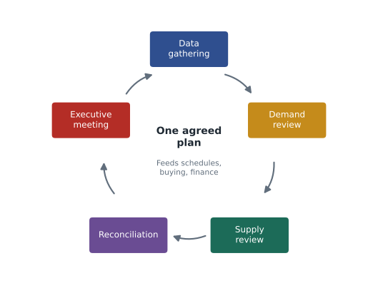
A typical cycle has five steps. First, data are gathered and the statistical forecast is updated after the month closes. Second, a demand review brings sales, marketing and planning together to agree an unconstrained demand plan, with assumptions and risks stated. Third, a supply review checks the demand plan against capacity, suppliers and inventory and identifies constraints and options. Fourth, a reconciliation meeting, sometimes called pre-S&OP, prepares scenarios and recommendations on the issues that need decisions, with their financial effects. Fifth, the executive meeting, chaired by the chief executive, makes those decisions and approves the plan. The meeting is short because the work has been done in advance; its value lies in making trade-offs explicit and owned, rather than leaving them to be settled by default in the warehouse.

Aggregate planning

At the heart of the supply review is aggregate planning: deciding how to meet a seasonal or uneven demand plan with production, workforce, overtime, subcontracting and inventory. Two pure strategies frame the choice. A chase strategy changes output each month to match demand, which keeps inventory low but incurs the costs of hiring and laying off workers, overtime and idle time, and can damage quality and morale. A level strategy produces at a constant rate and lets inventory absorb the difference, building stock in slow months and drawing it down in busy ones, which keeps the workforce stable but carries inventory and the risk of obsolescence. Services cannot store output, so they must chase with staffing or manage demand. Most firms choose a mixed strategy, changing the rate a few times a year.

Daniel models the brackets Northfield makes for agricultural equipment makers, whose demand peaks in spring as equipment is built for the planting season. Monthly demand runs from 28,000 in August to 60,000 in April, totaling 520,000 a year. Holding a bracket in stock costs about 30 cents a month, and every change in the production rate of 1,000 brackets a month costs about 1,200 dollars in hiring, training, layoffs and lost productivity. The code compares the pure strategies with a two-rate plan.

demand = [42, 48, 55, 60, 52, 40, 30, 28, 35, 40, 44, 46]   # thousands of brackets, January to December
hold, change = 0.30, 1.20   # thousand dollars per thousand units held a month, per thousand units of rate change

def plan_cost(rates):
    inv, low = 0, 0
    for r, d in zip(rates, demand):
        inv += r - d
        low = min(low, inv)
    start = -low                      # opening stock needed to avoid any shortage
    inv, holding = start, 0
    for r, d in zip(rates, demand):
        inv += r - d
        holding += inv * hold
    changes = sum(abs(rates[i] - rates[i - 1]) for i in range(12)) * change
    return holding, changes, start

plans = {'Chase': demand, 'Level': [sum(demand) / 12] * 12}
best = min(((a, b) for a in range(40, 61) for b in range(28, 46) if 5 * a + 7 * b >= sum(demand)),
           key=lambda ab: sum(plan_cost([ab[0]] * 5 + [ab[1]] * 7)[:2]))
plans[f'Two rates ({best[0]} then {best[1]})'] = [best[0]] * 5 + [best[1]] * 7
for name, rates in plans.items():
    h, c, s = plan_cost(rates)
    print(f"{name:22} holding {h:5.1f}  rate changes {c:5.1f}  total {h + c:5.1f}  opening stock {s:4.1f}")

Chase                  holding   0.0  rate changes  86.4  total  86.4  opening stock  0.0
Level                  holding  99.6  rate changes   0.0  total  99.6  opening stock 40.3
Two rates (51 then 38) holding  39.0  rate changes  31.2  total  70.2  opening stock  4.0

The level plan avoids all rate changes but must start the year with about 40,000 brackets in stock to cover the spring peak, and holding costs come to almost 100,000 dollars. The chase plan carries no inventory but changes rate every month, at a cost of about 86,000 dollars. The best two-rate plan, producing 51,000 a month from January to May and 38,000 for the rest of the year, costs about 70,000 dollars, less than either pure strategy. Real plans add constraints, such as overtime limits, minimum crew sizes and the risk that customers' spring orders change, which is exactly what the supply review discusses.

From the aggregate plan to the schedule

S&OP sits at the top of a planning hierarchy. Below it, the master production schedule converts the aggregate plan for product families into quantities of specific items by week. Material requirements planning, MRP, developed in the 1960s and described by Joseph Orlicky in a 1975 book, then works backward from the master schedule through the bill of materials, the list of components in each product, to calculate what parts and materials to order or make and when, offsetting each by its lead time. Below MRP sits detailed scheduling of machines and people. Enterprise resource planning systems integrate these steps with purchasing, inventory and finance. In a lean plant, MRP may plan materials over longer horizons while kanban controls day-to-day production, combining push for planning with pull for execution.

For Cedarline, the cohort proposes a simple first S&OP cycle. It would forecast at the level of product families, such as insulated jackets, shells, fleece and footwear, by channel, for 18 months. Merchandising, finance, the distribution center and the website team would agree one demand plan each month, with an upside and a downside. Buys would be committed in stages as the season approaches, which lesson 12 develops. And the executive team would review the plan monthly against inventory and margin targets. Dr. Raman warns that the hardest part will not be the spreadsheet. It will be persuading the chief executive that the agreed forecast is a forecast, not a target, and that the two must be kept separate.