
MBA-513 · Lesson 12 of 12 · 24 min
Capstone: redesigning Cedarline's supply chain
For the final two sessions, the cohort works in teams on a single brief from Cedarline's board. The company has agreed to the working-capital plan from Corporate Finance and the marketing plan from Marketing Management, which together cut promotions, prune the assortment from about 3,400 to about 2,400 styles and variants and stage the opening of new stores. The board now wants the supply chain that can deliver those plans: one that holds far less inventory, sells more at full price and copes with an uncertain trading environment. Dr. Raman gives the teams the same data the cohort has used all term and asks for a design, the numbers behind it and a plan for putting it in place. She reminds them that a supply chain redesign is not a single decision but a set of linked choices, each of which this course has examined on its own.
The diagnosis
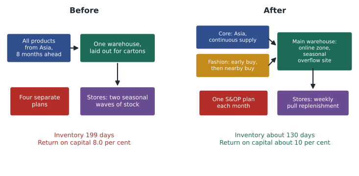
The teams begin by restating what lessons 1 to 11 revealed. Cedarline's inventory equals about 199 days of cost of goods sold, up from 147 four years ago, and its return on invested capital of 8.0 percent is below its 9 percent cost of capital. Its value stream map shows a lead time of about 205 days from purchase order to sale, of which about five and a half days add value. It buys every product the same way, eight months ahead, from Asian factories, although about 40 percent of revenue comes from functional products with predictable demand and 60 percent from innovative products whose demand is highly uncertain. Four functions plan on four different numbers. Its single distribution center was laid out for cartons and now handles a quarter of its volume as individual online orders, picked with a defect rate of about four sigma. And its exposure to a single membrane mill in Taiwan could cost it more than 10 million dollars of margin in a bad season.
Each problem has a familiar cause. The long, uniform lead time forces the merchandising team to commit to detailed quantities, by style, shade and size, when forecasts are least accurate, so errors are large. Buying to sales targets rather than to forecasts, with an implied critical ratio far above what the economics justify, inflates the buy. Leftover stock is cleared by promotions that lower the true salvage value and train customers to wait. The four plans mean the distribution center and the website cannot prepare for what merchandising buys. And the lack of multi-tier visibility hides concentration risk. Dr. Raman summarizes it in one sentence: Cedarline has an efficient supply chain for an innovative business.
Segmenting the supply chain
The teams' first design choice follows Fisher's framework from lesson 10: run two supply chains rather than one. For functional products, the core fleeces, base layers, socks and basic shells that sell year after year, Cedarline should keep its efficient Asian supply base and make it more efficient. These items should move from seasonal buys to continuous replenishment, with economic order quantities, reorder points and safety stock set as in lesson 9, full containers and long production runs agreed with the factories in return for steady volume. Their demand is predictable enough that an eight-month lead time costs little.
For innovative products, the seasonal jackets and fashion shades, Cedarline should build a responsive chain. Three tools work together. The first is staged commitment: buy part of the season's forecast early from Asia at low cost and hold back the rest for a second buy, placed after the first three weeks of sales, from a nearby factory in Mexico or Central America that can deliver within five weeks. The second is postponement: hold undyed or standard-shade fabric at the mills, so that the second buy can be cut and sewn in whatever shades early sales favor. The third is ordering by the economics of each item, using the newsvendor's critical ratio with a realistic salvage value rather than the sales target. The teams test the first and third tools together on Cedarline's winter parka.
import random
from statistics import NormalDist
N = NormalDist()
rng = random.Random(2026)

price, salvage = 289, 40          # full price; effective salvage of leftover parkas
asia, near = 120, 135             # landed cost: Asian early buy, nearby second buy
mu, sd_total, sd_late = 8000, 2400, 900
sd_early = (sd_total ** 2 - sd_late ** 2) ** 0.5   # uncertainty resolved by early sales
draws = [(N.inv_cdf(rng.random()) * sd_early, N.inv_cdf(rng.random()) * sd_late)
         for _ in range(20000)]

def profit(q_asia, q_near, d):
    sold = min(d, q_asia + q_near)
    return price * sold + salvage * (q_asia + q_near - sold) - asia * q_asia - near * q_near, sold

# Option 1: one buy from Asia, set by the newsvendor critical ratio
q1 = mu + N.inv_cdf((price - asia) / (price - salvage)) * sd_total
res = [profit(q1, 0, max(0, mu + a + b)) for a, b in draws]
p1 = sum(r[0] for r in res) / len(res)
left1 = sum(q1 - r[1] for r in res) / len(res)
print(f"Single buy: {q1:,.0f} units, expected profit {p1:,.0f}, leftover {left1:,.0f}")

# Option 2: early buy from Asia, then a second buy once early sales reveal part of demand
z2 = N.inv_cdf((price - near) / (price - salvage))
def staged(qa):
    tot = left = extra = 0
    for a, b in draws:
        qn = max(0, mu + a + z2 * sd_late - qa)
        p, s = profit(qa, qn, max(0, mu + a + b))
        tot += p; left += qa + qn - s; extra += qn
    n = len(draws)
    return tot / n, left / n, extra / n

best = max(range(3000, 9001, 250), key=lambda q: staged(q)[0])
p2, left2, extra2 = staged(best)
print(f"Staged: early buy {best:,}, average second buy {extra2:,.0f}, expected profit {p2:,.0f}, leftover {left2:,.0f}")
print(f"Gain {p2 - p1:,.0f} ({p2 / p1 - 1:.1%}); leftover stock cut by {1 - left2 / left1:.0%}")Single buy: 9,114 units, expected profit 1,136,723, leftover 1,621 Staged: early buy 6,500, average second buy 2,031, expected profit 1,224,584, leftover 749 Gain 87,861 (7.7%); leftover stock cut by 54%
The simulation draws 20,000 possible seasons. With a single buy set at the critical ratio, Cedarline would order about 9,100 parkas and expect about 1,600 to be left over. With staged commitment, the best early buy is about 6,500 parkas, roughly four-fifths of the forecast, and the second buy averages about 2,000 more, placed only when early sales show which way the season is going. Although the second buy costs 15 dollars more per parka, expected profit rises by about 88,000 dollars, nearly 8 percent, and leftover stock falls by more than half, to about 750 parkas. Across the roughly 280 million dollars of revenue from innovative products, the teams estimate that staged buying and better order quantities could cut markdowns by enough to add about 1.6 points to the company's gross margin, before the extra cost of nearby production.
Planning: one number
The second design choice is the S&OP process of lesson 8. The teams propose that Cedarline's chief operating officer, a role the leadership diagnosis in MBA-503 recommended creating, chair a monthly executive meeting that approves one plan by product family and channel for the next 18 months. The demand review would start from statistical forecasts by family, with merchandising and marketing adding known events such as product launches and the reduced promotion calendar from the marketing plan, and every adjustment would be tested for forecast value added. The supply review would translate the plan into early and second buys, factory capacity reservations, distribution center staffing and third-party warehouse space. Finance would attach the plan's inventory, margin and cash implications. The chief executive's growth ambition would be kept as a target, reported beside the forecast but not used to buy against.
Two metrics would anchor the process. Forecast accuracy and bias by family, with tracking signals, would show whether the plan is trustworthy. Full-price sell-through, the share of units sold before any markdown, would show whether the buys match demand. The teams set targets of reducing the forecast error at the family level from about 34 percent to about 24 percent within two seasons, the improvement the cohort estimated in MBA-504, and raising full-price sell-through from about 62 percent to about 72 percent.
The distribution center and stores
The third choice concerns the physical network. The teams recommend against building the second distribution center now. Lesson 10's network model showed that one and two buildings cost almost the same, and lesson 3 showed that the existing building's main problem is its layout, not its size. They propose three changes inside the building: slot items by pick frequency, which cuts picker walking by more than half; create a separate zone with its own packing stations for online orders; and install barcode scanning at the pick face, a poka-yoke that should move picking accuracy from about four sigma toward five. A third-party warehouse near the main market would handle seasonal overflow from September to December under a variable-cost contract. The board would revisit the second building, as an option, once online volume passes a set threshold or delivery speed becomes an order winner.
Store replenishment would change from seasonal allocations to weekly pull. Rather than pushing most of a season's stock to stores in two large waves, the distribution center would hold more of it and replenish each store weekly to an order-up-to level based on that store's own sales. Lesson 9's square-root law shows why this cuts inventory: safety stock held in one place covers the combined variability of 62 stores far more cheaply than safety stock in each store. Online orders could also be filled from store stock when the distribution center runs out, pooling inventory across channels. The cost is more frequent store deliveries, which the teams estimate at about 0.4 million dollars a year in extra freight, included in their figures below.
Quality, suppliers and risk
The fourth set of choices concerns suppliers. Cedarline would reduce the number of factories it uses for innovative products and build deeper relationships, in the manner Liker and Choi described, with the two or three that will hold reactive capacity and fabric for it. In return for that commitment, the factories would agree to inline quality checks with p charts shared with Cedarline, as in lesson 4, rather than final inspection alone, and to notify Cedarline before changing machines or materials, the special cause behind lot 10's defects. For the membrane fabric, the teams recommend holding five more weeks of stock immediately, which closes half of the gap between time to recover and time to survive found in lesson 11 at modest cost, and starting qualification of a second mill for the following year. They also propose mapping the supply chain to the second tier for every strategic and bottleneck item in Kraljic's matrix, which would also support Cedarline's forced labor reporting.
The trade environment shapes the sourcing split. Because Asian imports now carry high ordinary duties plus the additional duties of 2026, while Mexican production from North American fabric enters duty-free under the agreement, the teams shift some core styles to Mexico as well, not just the responsive fashion volume, and model the remaining Asian core volume with a duty assumption that the customs broker must confirm. The annual reviews of the agreement add uncertainty, so contracts with Mexican factories would include volume flexibility rather than long fixed commitments.
The financial case
# Cedarline supply chain plan: steady-state effect by fiscal 2029 (millions of dollars)
revenue, gm0, tax, wacc = 468.0, 0.498, 0.265, 0.09
nopat0 = 39.8 * (1 - tax)
ic0 = nopat0 / 0.080
inv0 = 128.0

margin_points = 1.6 - 0.5 + 0.2      # fewer markdowns, nearby production premium, less air freight
gm1 = gm0 + margin_points / 100
opex = 1.0 + 0.6 + 0.4 + 0.4 + 0.2 - 1.5   # overflow warehouse, planning team, membrane stock,
                                           # store freight, scanning support, less picking savings
capex = 4.5                                # online zone, scanners, slotting project
days1 = 130
inv1 = revenue * (1 - gm1) * days1 / 365

nopat1 = nopat0 + (revenue * margin_points / 100 - opex) * (1 - tax)
ic1 = ic0 - (inv0 - inv1) + capex
print(f"Gross margin {gm0:.1%} -> {gm1:.1%}; inventory {inv0:.0f} -> {inv1:.1f} ({days1} days)")
print(f"Cash released from inventory, net of capital spending: {inv0 - inv1 - capex:.1f}")
print(f"NOPAT {nopat0:.1f} -> {nopat1:.1f}; invested capital {ic0:.0f} -> {ic1:.0f}")
print(f"ROIC {nopat0 / ic0:.1%} -> {nopat1 / ic1:.1%} against a cost of capital of {wacc:.0%}")
ep0, ep1 = nopat0 - wacc * ic0, nopat1 - wacc * ic1
print(f"Economic profit {ep0:+.1f} -> {ep1:+.1f} a year")Gross margin 49.8% -> 51.1%; inventory 128 -> 81.5 (130 days) Cash released from inventory, net of capital spending: 42.0 NOPAT 29.3 -> 32.9; invested capital 366 -> 324 ROIC 8.0% -> 10.2% against a cost of capital of 9% Economic profit -3.7 -> +3.8 a year
The output shows why the board should care. With gross margin up by about 1.3 points net of the cost of nearby production, and inventory down from 128 to about 82 million dollars, or 130 days of cost of goods sold, the plan releases about 42 million dollars of cash after its capital spending. After-tax operating profit rises from about 29 to about 33 million dollars, invested capital falls from about 366 to about 324 million, and return on invested capital rises from 8.0 to about 10.2 percent, above the cost of capital for the first time since fiscal 2023. Economic profit swings from about minus 3.7 million dollars a year to about plus 3.8 million. The teams are careful about overlap with the marketing plan: the assortment pruning agreed there is one of the reasons inventory can fall, so they do not add the marketing plan's margin gains to these figures, which would count the same improvement twice.
| Area | Change | Main lessons |
|---|---|---|
| Assortment | Two supply chains: efficient for functional, responsive for innovative | 1, 10 |
| Buying | Staged commitment, postponement, newsvendor quantities | 9, 12 |
| Planning | Monthly S&OP with one plan; forecast kept separate from target | 8 |
| Distribution center | Slotting, online zone, scanning, overflow warehouse; defer second building | 2, 3, 6, 7, 10 |
| Stores | Weekly pull replenishment, pooled stock across channels | 5, 9 |
| Suppliers | Fewer, deeper relationships; inline quality; second-tier mapping | 4, 10, 11 |
| Risk | Extra membrane stock now; second mill qualified next year | 11 |
Making it happen
The teams' implementation plan runs over two years and starts with what is cheapest and most certain. In the first six months: start the monthly S&OP cycle, re-slot the distribution center, install pick-face scanning, buy the extra membrane stock and move the core products to continuous replenishment. In the next six months, before the following winter's buy: pilot staged commitment on about 20 fashion styles with one Mexican partner, measure the results against matched styles bought the old way, as the cohort learned to do in MBA-504, and open the online zone. In the second year: extend staged buying to the styles where the pilot pays, qualify the second membrane mill, move store replenishment to weekly pull and reach the inventory target. Each step has an owner, a metric and a decision point at which the board can stop or continue, in the spirit of the staged investments the cohort valued in Corporate Finance.
Dr. Raman's closing comments return to the photograph of the two loading docks from the first session. The quiet dock, she says, belonged to a company that had learned to see its supply chain as one system, flowing at the pace of demand, with problems surfaced rather than buried in inventory. Cedarline's dock today has trucks waiting at the gate and cartons stacked to the ceiling, and its accounts show the result. The redesign will not make Cedarline's demand any more predictable. What it does is arrange the company so that it commits later, learns faster and pays for uncertainty only where uncertainty is real. That, she says, is what operations strategy means.
Worked problem
Choosing which styles to stage
Cedarline has capacity at its Mexican partner for second buys on about 60 fashion styles next winter. The merchandising team proposes choosing the 60 styles with the highest expected sales. A team member suggests instead choosing the styles with the highest forecast uncertainty relative to their margin. Use the logic of the capstone to decide.
Show solution
- The value of staging comes from learning: buying after early sales reveal part of demand. A style with predictable demand gains little from a second buy, however large its sales.
- The value also depends on the margin at stake: the gap between full price and landed cost, and between landed cost and salvage, sets the costs of underage and overage.
- A useful ranking multiplies the uncertainty resolved by early sales, the standard deviation of demand that early sales would reveal, by the margin, giving roughly the expected cost of mismatch that staging can avoid.
- Styles with large, predictable sales should be bought early from Asia; staged capacity should go to styles that are both uncertain and profitable, even if their expected sales are smaller.
Answer: Reactive capacity is scarce and should be allocated where it buys the most information. Choosing by expected sales alone would put it on the styles that need it least.
Common mistakes
MistakeA redesign means changing everything at once.
InsteadStart with low-cost, high-certainty changes, pilot the uncertain ones and stage the rest with decision points.
MistakeA responsive supply chain is always more expensive.
InsteadIts higher production costs can be more than offset by fewer markdowns and less inventory.
MistakeThe second distribution center is needed because the building is full.
InsteadThe layout, not the size, is the main constraint; overflow can be handled flexibly while the option is kept open.
MistakeSupply chain gains can be added to marketing and finance gains.
InsteadOverlapping improvements must not be counted twice; integrate the plans.
Summary and key terms
- Cedarline's diagnosis: an efficient, uniform supply chain serving a largely innovative business, with long lead times, buying to targets and four plans.
- Two supply chains: continuous replenishment from Asia for functional products; staged commitment, postponement and nearby second buys for innovative ones.
- Staged commitment on the parka raises expected profit by about 8 percent and halves leftover stock.
- One S&OP plan, with forecasts separated from targets and measured by accuracy, bias and full-price sell-through.
- Distribution center layout, scanning and overflow capacity instead of a second building now; weekly pull to stores.
- The plan lifts ROIC from 8.0 to about 10.2 percent and turns economic profit positive, and is implemented in stages with pilots.
- Staged commitment
- Buying part of a season early and the rest after early sales reveal demand.
- Reactive capacity
- Production capacity held to fill second buys quickly during the season.
- Full-price sell-through
- The share of units sold before any markdown.
- Continuous replenishment
- Regular reordering of stable products based on actual consumption.
- Economic profit
- NOPAT minus the cost of capital times invested capital.
- Supply chain segmentation
- Running different supply chains for products with different demand and supply characteristics.
Practice problems
Work each problem on paper first, then reveal the answer to check.
Why does the best early buy in the staged plan fall below the mean forecast?
Show answer
Because a second buy is available after demand becomes clearer, the early buy only needs to cover the likely minimum; holding back reduces leftover stock.
If the nearby factory's landed cost rose from 135 to 160 dollars, how would the staged plan change?
Show answer
The second buy's critical ratio would fall, so it would be smaller, the early buy larger, and the gain from staging smaller.
Inventory falls from 128 to 82 million dollars and the plan spends 4.5 million of capital. By how much does invested capital fall?
Show answer
128 - 82 - 4.5 = 41.5 million dollars.
Name two metrics the S&OP process should track and explain why.
Show answer
Forecast accuracy and bias, to show whether the plan can be trusted; full-price sell-through, to show whether buys match demand.
Lesson quiz · 5 questions
Score 60% or more to complete this lesson.
Create a free account to save your progress, take quizzes and earn a certificate.