Stochastic models: Markov chains and Monte Carlo simulation

The models so far have been deterministic: the same inputs always give the same outputs. Real systems are subject to chance. Whether the first influenza case in a small town infects anyone, whether a bus meets a slow passenger, whether a spring is warm enough for walleye eggs to hatch, are all matters of luck, and when numbers are small luck dominates. This lesson introduces two of the main tools for stochastic modeling. Markov chains describe systems that jump between states with fixed probabilities and can be analyzed exactly with matrices. Monte Carlo simulation estimates the behavior of any stochastic model by running it many times, and comes with a simple rule for its own accuracy.

Random events in models

A stochastic model specifies probabilities rather than certainties. The basic building blocks are random variables with known distributions. Arrivals of passengers at a stop are often modeled as a Poisson process with rate \(\lambda\): the number of arrivals in a time interval of length \(t\) has the Poisson distribution with mean \(\lambda t\), \[\Pr(k \text{ arrivals}) = \frac{(\lambda t)^ke^{-\lambda t}}{k!},\] and the gaps between arrivals are independent exponential random variables with mean \(\frac{1}{\lambda}\). This is the natural model when arrivals come from many independent people, each unlikely to arrive in any short interval. The exponential distribution also lies behind the constant recovery rate \(\gamma\) of the SIR model: it is the only continuous distribution for which the chance of recovering in the next hour does not depend on how long one has been ill.

The deterministic models of earlier lessons can be viewed as describing the averages of stochastic ones when numbers are large. A population of 40,000 walleye with random individual births and deaths has fluctuations of order \(\sqrt{40{,}000} = 200\), half a percent, which the logistic model rightly ignores. A town with three infected people has fluctuations as large as the numbers themselves, and the deterministic model can be badly misleading.

Markov chains

A discrete-time Markov chain is a sequence of random states \(X_0, X_1, X_2, \dots\) taking values in a finite set \(\{1, \dots, m\}\), with the Markov property: the probability of the next state depends only on the current state, not on the earlier history. The chain is described by its transition matrix \(P\), with entries \[P_{ij} = \Pr(X_{t+1} = j \mid X_t = i).\] Each row of \(P\) is a probability distribution, so its entries are nonnegative and sum to 1. If the row vector \(p^{(t)}\) gives the probabilities of the states at time \(t\), then \(p^{(t+1)} = p^{(t)}P\) and \(p^{(t)} = p^{(0)}P^t\). The difference equation methods of lesson 4 thus apply to probability distributions.

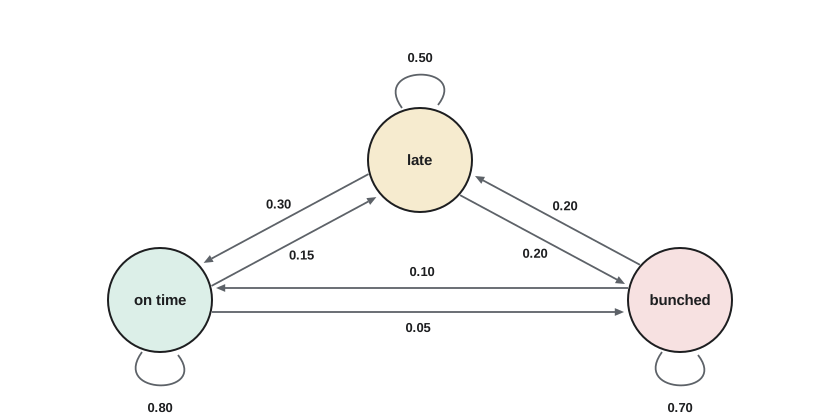
The transit agency classifies each Route 9 bus, as it passes a timing point, into one of three states: on time (state 1), late by up to 4 minutes (state 2) and bunched with the bus ahead (state 3). From automatic vehicle location records it estimates the transition probabilities between successive timing points: \[P = \begin{pmatrix} 0.80 & 0.15 & 0.05 \\ 0.30 & 0.50 & 0.20 \\ 0.10 & 0.20 & 0.70 \end{pmatrix}.\] A bus on time stays on time with probability 0.8; a bunched bus stays bunched with probability 0.7, reflecting the instability studied in lesson 4.

Stationary distributions

After many steps, how likely is a bus to be in each state? A distribution \(\pi\) is stationary if \(\pi P = \pi\): once the chain has this distribution it keeps it. Equivalently \(\pi\) is a left eigenvector of \(P\) with eigenvalue 1, normalized so its entries sum to 1.

Theorem 9.1. If some power of \(P\) has all entries positive, then the chain has a unique stationary distribution \(\pi\), and for every initial distribution \(p^{(0)}\), \(p^{(0)}P^t \to \pi\) as \(t \to \infty\). Moreover the long-run fraction of time the chain spends in state \(j\) equals \(\pi_j\). This is a form of the Perron–Frobenius theorem: 1 is the largest eigenvalue of \(P\), all other eigenvalues have absolute value less than 1, and the convergence is geometric at the rate of the second largest eigenvalue in absolute value.

The model now supports decisions. If headway control at timing points, as designed in lesson 4, changes the probability of leaving the bunched state from 0.3 to 0.5, the stationary distribution can be recomputed to predict the improvement. The mean number of timing points a bunched bus stays bunched is \(\frac{1}{1 - 0.7} \approx 3.3\), since the time spent in a state is geometric, and the control would reduce this to 2.

Branching processes and the chance of an outbreak

At the start of an epidemic each infectious person causes a random number of new cases, independently of the others. A model with this structure is a branching process. Let the number of secondary cases caused by one case have mean \(R_0\) and probability generating function \(G(s) = \sum_k p_ks^k\), where \(p_k\) is the probability of exactly \(k\) secondary cases. The probability \(q\) that the chain of transmission started by one case eventually dies out is the smallest nonnegative root of \[q = G(q).\] The reasoning is that the chain dies out exactly when each of the first case's offspring starts a chain that dies out, and these events are independent.

If \(R_0 \le 1\), the only root in \([0, 1]\) is \(q = 1\): extinction is certain. If \(R_0 > 1\), there is a root \(q < 1\), and a major outbreak occurs with probability \(1 - q\). In the SIR model with exponentially distributed infectious periods, the number of secondary cases is geometric with \(G(s) = \frac{1}{1 + R_0(1 - s)}\), and solving \(q = G(q)\) gives \(q = \frac{1}{R_0}\). So a single case starts a major outbreak with probability \(1 - \frac{1}{R_0}\), and with \(k\) initial cases the probability is \(1 - R_0^{-k}\). For influenza with \(R_0 = 1.5\), a single introduction fizzles out two times in three, which is why the start of an epidemic in a new place is so unpredictable.

Monte Carlo simulation

For most stochastic models, exact formulas like those above are not available. Monte Carlo simulation estimates any quantity of interest by simulating the model many times with random numbers and averaging. If \(Y\) is a random output, such as the final size of an outbreak, and \(Y_1, \dots, Y_n\) are independent simulated values, the estimate is the sample mean \(\bar{Y} = \frac{1}{n}\sum Y_k\). The law of large numbers guarantees \(\bar{Y} \to E[Y]\), and the central limit theorem gives its accuracy: \(\bar{Y}\) is approximately normal with standard deviation \(\frac{\sigma}{\sqrt{n}}\), where \(\sigma\) is the standard deviation of \(Y\). An approximate 95% confidence interval is \[\bar{Y} \pm 1.96\frac{s}{\sqrt{n}},\] with \(s\) the sample standard deviation.

The \(\frac{1}{\sqrt{n}}\) rule is the great strength and the main weakness of Monte Carlo. It holds whatever the complexity of the model, in any number of dimensions, so the method applies to models far too complicated for exact analysis. But it converges slowly: each extra decimal digit of accuracy needs a hundred times as many runs. Estimating a probability \(p\) has standard error \(\sqrt{\frac{p(1 - p)}{n}}\), so to estimate a probability near 0.3 to within \(\pm 0.01\) needs roughly 8000 runs.

A stochastic epidemic in a small town

The program below simulates the SIR model as a stochastic process in a town of 1000 people with one initial case. Events happen one at a time: an infection occurs at rate \(\frac{\beta SI}{P}\) and a recovery at rate \(\gamma I\). Since only the sequence of events matters for the final size, each event is an infection with probability \(\frac{\beta S/P}{\beta S/P + \gamma}\) and a recovery otherwise. This is the embedded jump chain of the continuous-time process, a Markov chain on the states \((S, I)\).

import random, math
random.seed(424)

def final_size(P=1000, R0=1.5, I0=1):
    S, I, total = P - I0, I0, I0
    while I > 0:
        p_inf = R0 * S / P / (R0 * S / P + 1)    # gamma = 1 after scaling time
        if random.random() < p_inf:
            S -= 1; I += 1; total += 1
        else:
            I -= 1
    return total

runs = 4000
sizes = [final_size() for _ in range(runs)]
major = [z for z in sizes if z > 100]
p_hat = len(major) / runs
se = math.sqrt(p_hat * (1 - p_hat) / runs)
print(f"P(major outbreak) = {p_hat:.3f} +/- {1.96 * se:.3f}   (theory 1 - 1/R0 = {1 - 1 / 1.5:.3f})")
print(f"mean size of minor outbreaks: {sum(z for z in sizes if z <= 100) / (runs - len(major)):.2f} people")
mean_major = sum(major) / len(major)
print(f"mean final fraction in major outbreaks: {mean_major / 1000:.3f}  (deterministic 0.583)")
print("histogram of final sizes:")
for lo in range(0, 1000, 100):
    n = sum(lo <= z < lo + 100 for z in sizes)
    print(f"  {lo:4d}-{lo + 99:4d}: {n:5d} " + "#" * (n // 50))

P(major outbreak) = 0.318 +/- 0.014   (theory 1 - 1/R0 = 0.333)
mean size of minor outbreaks: 3.23 people
mean final fraction in major outbreaks: 0.579  (deterministic 0.583)
histogram of final sizes:
     0-  99:  2727 ######################################################
   100- 199:     2 
   200- 299:     3 
   300- 399:    13 
   400- 499:    97 #
   500- 599:   632 ############
   600- 699:   514 ##########
   700- 799:    12 
   800- 899:     0 
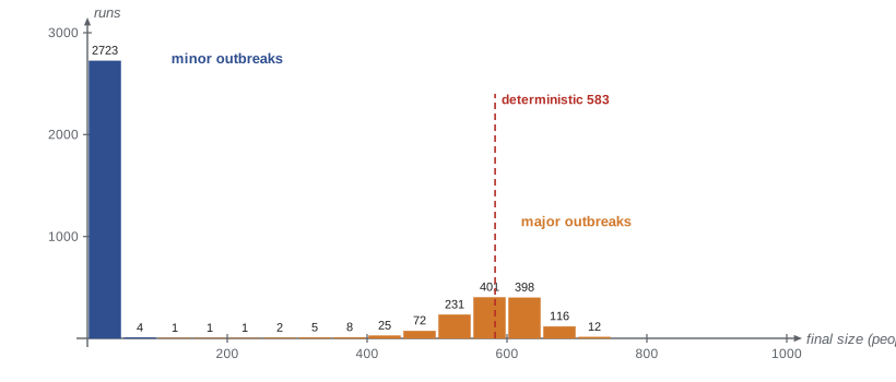
   900- 999:     0

The results show the two faces of the stochastic model. About two thirds of introductions die out after infecting only a handful of people, three on average, and the estimated probability of a major outbreak, about 0.32, is close to the branching process prediction \(1 - \frac{1}{R_0} = \frac{1}{3}\); the small difference reflects the finite town, in which susceptible people are depleted even during the early phase. When an outbreak does take off, its final size is close to the deterministic value of 58%, with modest scatter. The distribution of outcomes is bimodal, which a deterministic model cannot represent. For the health unit, this means that early in the season, with few cases, forecasts should be stated as probabilities.

Randomness in the fishery

Walleye recruitment varies greatly from year to year with spring water temperatures and wind. A stochastic version of the Ricker model of lesson 4 multiplies recruitment by a random factor: \(N_{t+1} = N_te^{r(1 - N_t/K) + \sigma Z_t}\), where the \(Z_t\) are independent standard normal variables and \(\sigma\) measures environmental variability. Monte Carlo simulation of this model answers questions such as: what is the probability that the stock falls below 10,000 within 20 years under a given harvest rule? Such risk-based questions, rather than single deterministic predictions, are now the standard form of advice in fisheries management, and they bring together the models of lessons 4, 5 and 8 with the stochastic tools of this lesson.