Scaling, nondimensionalization and small parameters

Lesson 2 showed that the answer to a physical question can always be written in terms of dimensionless groups. This lesson turns that idea into a working technique for differential equation models. Nondimensionalization rewrites a model in dimensionless variables, chosen so that the important terms have size about one. The result has fewer parameters, reveals which combinations of parameters control the behavior, and exposes small parameters that can be exploited by approximation. We apply it to the fishery, to the influenza model and to a classical problem of projectile motion.

Choosing scales

Every dimensional variable is the product of a dimensionless variable and a scale with the same units. For the fish population we write \(N = N_c x\), where \(N_c\) is a characteristic population, and for time \(t = t_c\tau\), where \(t_c\) is a characteristic time. The scales are not given by the problem; we choose them, and a good choice is one that makes the new variables \(x\) and \(\tau\) of order one in the regime of interest, and their derivatives of order one as well.

There are usually natural candidates. A population with a carrying capacity has the natural scale \(K\); a process with a rate \(r\) has the natural time scale \(\frac{1}{r}\); a pendulum has the length \(\ell\) and the time \(\sqrt{\frac{\ell}{g}}\). When several candidates exist, the choice depends on which process we want to resolve, and different choices lead to different approximations. Choosing scales is therefore a modeling decision, not a mechanical step.

Nondimensionalizing the fishery

Start from the harvested logistic model of lesson 1: \[\frac{dN}{dt} = rN\Big(1 - \frac{N}{K}\Big) - H.\] It has three parameters, \(r\), \(K\) and \(H\). Substitute \(N = Kx\) and \(t = \frac{\tau}{r}\). By the chain rule \(\frac{dN}{dt} = \frac{d(Kx)}{d\tau}\frac{d\tau}{dt} = Kr\frac{dx}{d\tau}\). Dividing the equation by \(Kr\) gives \[\frac{dx}{d\tau} = x(1 - x) - h, \qquad h = \frac{H}{rK}.\]

The model now has a single parameter \(h\), the catch measured in units of \(rK\). Every fishery described by this model, whatever its size and growth rate, behaves the same way for the same \(h\). Lesson 5 shows that \(h = \frac{1}{4}\) is the critical value; in dimensional terms the maximum sustainable catch is \(\frac{rK}{4}\), which for Larch Lake is \(\frac{0.3 \times 40{,}000}{4} = 3000\) fish per year. The dimensionless form tells us at a glance that doubling the carrying capacity doubles the safe catch, and so does doubling the growth rate.

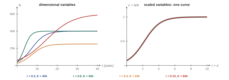
The figure illustrates the general principle. Without scaling, a parameter study of the unharvested logistic model would require varying \(r\), \(K\) and the initial value \(N_0\), three dimensions. After scaling, only the ratio \(x_0 = \frac{N_0}{K}\) matters, and the curves for different \(r\) and \(K\) coincide. Experiments and simulations become far more efficient, because each one covers a whole family of dimensional situations.

A general recipe

Nondimensionalization of a differential equation model proceeds in four steps. Identify the dependent and independent variables and introduce scales for each, \(u = u_c\bar{u}\), \(t = t_c\bar{t}\). Substitute into the equations, using the chain rule for derivatives: \(\frac{du}{dt} = \frac{u_c}{t_c}\frac{d\bar{u}}{d\bar{t}}\) and \(\frac{d^2u}{dt^2} = \frac{u_c}{t_c^2}\frac{d^2\bar{u}}{d\bar{t}^2}\). Divide through by the coefficient of one chosen term, usually the one we expect to dominate. Finally choose the scales to make as many of the remaining coefficients equal to one as possible; those that cannot be removed are the dimensionless parameters of the model.

The number of parameters that remain agrees with the pi theorem. In the fishery model there are five quantities \(N, t, r, K, H\) with two dimensions, fish and time, giving three groups \(x\), \(\tau\) and \(h\). Two of these are variables, so one parameter remains.

This is a typical outcome. The dimensionless parameter that survives scaling is often the most important number in the model, with a direct interpretation. Here \(R_0\) is the product of the infection rate per case at the start of the outbreak, \(\beta P\), and the mean infectious period \(\frac{1}{\gamma}\). Lesson 7 shows that the epidemic grows if and only if \(R_0 s(0) > 1\).

Small parameters

Sometimes a dimensionless parameter is very small or very large. This is valuable information, because it suggests that one effect is weak and can be treated as a correction. If a scaled model has the form \(F(u, \varepsilon) = 0\) with \(\varepsilon \ll 1\), we may seek a solution as a series \[u = u_0 + \varepsilon u_1 + \varepsilon^2u_2 + \cdots,\] substitute, and collect powers of \(\varepsilon\). The leading term \(u_0\) solves the simplified problem with \(\varepsilon = 0\), and each correction solves a linear problem. This method is called regular perturbation.

Regular perturbation works when setting \(\varepsilon = 0\) leaves a problem of the same type. When it does not, for instance when \(\varepsilon\) multiplies the highest derivative, the method fails and the problem is called singular. A good choice of scales is what makes the small parameter visible in the first place, and different scales can make the same problem look regular in one region and singular in another.

The projectile problem

A ball is thrown straight up from the surface of the Earth with speed \(v_0\). If we account for the decrease of gravity with height \(y\), Newton's law gives \[\frac{d^2y}{dt^2} = -\frac{gR^2}{(R + y)^2}, \qquad y(0) = 0, \quad y^\prime(0) = v_0,\] where \(R\) is the radius of the Earth. How high does the ball go?

The obvious length scale \(R\) is a poor choice: the ball rises a few meters, so \(\frac{y}{R}\) is tiny and all the interesting motion is squeezed near zero. A better scale comes from the simple problem with constant gravity, where the ball rises to \(\frac{v_0^2}{2g}\) in time \(\frac{v_0}{g}\). So take \(y = \frac{v_0^2}{g}\bar{y}\) and \(t = \frac{v_0}{g}\bar{t}\). Substituting and simplifying gives \[\frac{d^2\bar{y}}{d\bar{t}^2} = -\frac{1}{(1 + \varepsilon\bar{y})^2}, \qquad \bar{y}(0) = 0, \quad \bar{y}^\prime(0) = 1, \qquad \varepsilon = \frac{v_0^2}{gR}.\]

For a ball thrown at 20 m/s, \(\varepsilon = \frac{400}{9.8 \times 6.37 \times 10^6} \approx 6.4 \times 10^{-6}\), very small. Setting \(\varepsilon = 0\) gives \(\bar{y}_0 = \bar{t} - \frac{\bar{t}^2}{2}\), the familiar parabola. To find the first correction, expand \((1 + \varepsilon\bar{y})^{-2} = 1 - 2\varepsilon\bar{y} + O(\varepsilon^2)\) and substitute \(\bar{y} = \bar{y}_0 + \varepsilon\bar{y}_1\). The terms of order \(\varepsilon\) give \(\bar{y}_1^{\prime\prime} = 2\bar{y}_0 = 2\bar{t} - \bar{t}^2\) with \(\bar{y}_1(0) = \bar{y}_1^\prime(0) = 0\), so \[\bar{y}_1 = \frac{\bar{t}^3}{3} - \frac{\bar{t}^4}{12}.\]

The program below checks the expansion against a careful numerical solution for several values of \(\varepsilon\). Since the error of a first-order expansion should be of order \(\varepsilon^2\), halving \(\varepsilon\) should cut the error by a factor of about four.

# Maximum height of the scaled projectile: y'' = -1/(1 + eps*y)^2, y(0)=0, y'(0)=1
def max_height(eps, dt=1e-4):
    y, v = 0.0, 1.0
    acc = lambda y: -1.0 / (1.0 + eps * y) ** 2
    while v > 0:                          # velocity Verlet until the ball stops rising
        a = acc(y)
        y_new = y + v * dt + 0.5 * a * dt * dt
        v_new = v + 0.5 * (a + acc(y_new)) * dt
        if v_new <= 0:                    # interpolate the turning point
            frac = v / (v - v_new)
            return y + frac * (y_new - y)
        y, v = y_new, v_new

print("  eps      numeric     1/2 + eps/4    error      exact")
for eps in [0.2, 0.1, 0.05, 0.025]:
    num = max_height(eps)
    approx = 0.5 + eps / 4
    exact = 0.5 / (1 - eps / 2)
    print(f"{eps:6.3f}   {num:.6f}    {approx:.6f}    {abs(exact - approx):.2e}   {exact:.6f}")

  eps      numeric     1/2 + eps/4    error      exact
 0.200   0.555556    0.550000    5.56e-03   0.555556
 0.100   0.526316    0.525000    1.32e-03   0.526316
 0.050   0.512821    0.512500    3.21e-04   0.512821
 0.025   0.506329    0.506250    7.91e-05   0.506329

The errors shrink by close to a factor of four each time \(\varepsilon\) halves, confirming that the approximation is correct to first order. For a real ball the correction is a few parts in a million, far smaller than the effect of air resistance, which is why the constant-gravity model is perfectly adequate for sports. For a rocket reaching orbital speeds, \(\varepsilon\) is close to 1 and the full model is needed. Scaling tells us in advance which regime we are in.

A singular problem and boundary layers

Consider \(\varepsilon u^{\prime\prime} + u^\prime = 1\) on \(0 < x < 1\) with \(u(0) = 0\) and \(u(1) = 2\), where \(\varepsilon\) is small. Setting \(\varepsilon = 0\) leaves \(u^\prime = 1\), a first-order equation that can satisfy only one boundary condition. The solution \(u = x + 1\) satisfies \(u(1) = 2\) but not \(u(0) = 0\). The exact solution, \[u(x) = x + \frac{1 - e^{-x/\varepsilon}}{1 - e^{-1/\varepsilon}},\] shows what happens: away from \(x = 0\) it is very close to \(x + 1\), but in a thin region of width about \(\varepsilon\) near \(x = 0\) it drops steeply to zero. This thin region is a boundary layer. Inside it the natural length scale is \(\varepsilon\), not 1, and rescaling \(x = \varepsilon X\) makes the second derivative term as large as the others.

Boundary layers are everywhere in applications: the thin layer of slow air next to an aircraft wing, the rapid initial phase of an enzyme reaction before it settles to a steady rate, and the first few days of an epidemic before the growth becomes exponential. The method of matched asymptotic expansions, developed in courses on perturbation methods, builds separate approximations inside and outside such layers and joins them. For this course the key lesson is diagnostic: if a small parameter multiplies the highest derivative, expect a region where the scales chosen for the rest of the problem are wrong.

Why scaling matters for computation

Nondimensionalization also helps numerical work. Variables of order one avoid overflow and loss of precision; time steps can be chosen relative to the natural time scale; and, most of all, a parameter study over a few dimensionless groups replaces a much larger study over dimensional parameters. When a scaled model contains both a very small and an ordinary parameter, it warns that the equations are stiff, with processes on very different time scales, and that an implicit numerical method may be needed.