Phase plane analysis: predator–prey and competition models

Walleye in Larch Lake do not live alone. Their main prey is yellow perch, and they compete with northern pike for the same food. Models of interacting species are systems of differential equations, and the phase line of lesson 5 becomes the phase plane. This lesson develops the tools for two-dimensional autonomous systems: nullclines, equilibria, linearization through the Jacobian matrix, and the classification of equilibria by trace and determinant. We apply them to the Lotka–Volterra predator–prey model, to a more realistic variant with limited prey, and to competition between two species.

Two-dimensional autonomous systems

A two-dimensional autonomous system has the form \[\frac{dx}{dt} = f(x, y), \qquad \frac{dy}{dt} = g(x, y),\] where \(f\) and \(g\) do not depend explicitly on \(t\). At each point of the \((x, y)\) plane the system specifies a velocity vector \((f, g)\), and a solution is a curve, called a trajectory or orbit, that follows these vectors. Under mild smoothness assumptions, trajectories cannot cross, since at a crossing point the velocity would have two values. The picture of all trajectories is the phase portrait.

Nullclines organize the phase portrait. The \(x\)-nullcline is the curve \(f(x, y) = 0\), on which trajectories move vertically; the \(y\)-nullcline is \(g(x, y) = 0\), on which they move horizontally. Equilibria are the intersections of the two nullclines. In each region bounded by nullclines the signs of \(f\) and \(g\) are constant, so the direction of motion is known to within a quadrant: up and right, up and left, and so on. Sketching nullclines and these directions is the first step of every phase plane analysis.

The Lotka–Volterra model

In the 1920s the mathematician Vito Volterra was asked by his son-in-law, the marine biologist Umberto D'Ancona, why the proportion of predatory fish in catches at Adriatic ports had risen during the First World War, when fishing was reduced. Alfred Lotka had proposed the same model independently. Let \(x\) be the prey, perch, and \(y\) the predators, walleye. In the absence of predators the prey grow exponentially; in the absence of prey the predators die out exponentially; and encounters, at a rate proportional to \(xy\), remove prey and add predators: \[\frac{dx}{dt} = ax - bxy, \qquad \frac{dy}{dt} = -cy + dxy,\] with positive constants \(a, b, c, d\).

The \(x\)-nullclines are \(x = 0\) and \(y = \frac{a}{b}\); the \(y\)-nullclines are \(y = 0\) and \(x = \frac{c}{d}\). So there are two equilibria: the origin and the coexistence point \((x^*, y^*) = (\frac{c}{d}, \frac{a}{b})\). In the positive quadrant, prey increase below the line \(y = \frac{a}{b}\) and decrease above it; predators increase to the right of \(x = \frac{c}{d}\) and decrease to the left. Following the directions around the coexistence point shows that trajectories circle it counterclockwise: prey increase, then predators increase, then prey decrease, then predators decrease.

In fact the trajectories are closed curves. Dividing the equations gives \(\frac{dy}{dx} = \frac{y(-c + dx)}{x(a - by)}\), which separates: \(\frac{a - by}{y}dy = \frac{-c + dx}{x}dx\). Integrating, the quantity \[V(x, y) = dx - c\ln x + by - a\ln y\] is constant along every trajectory. \(V\) has a strict minimum at \((x^*, y^*)\) and its level curves are closed loops around it, so every positive solution is periodic.

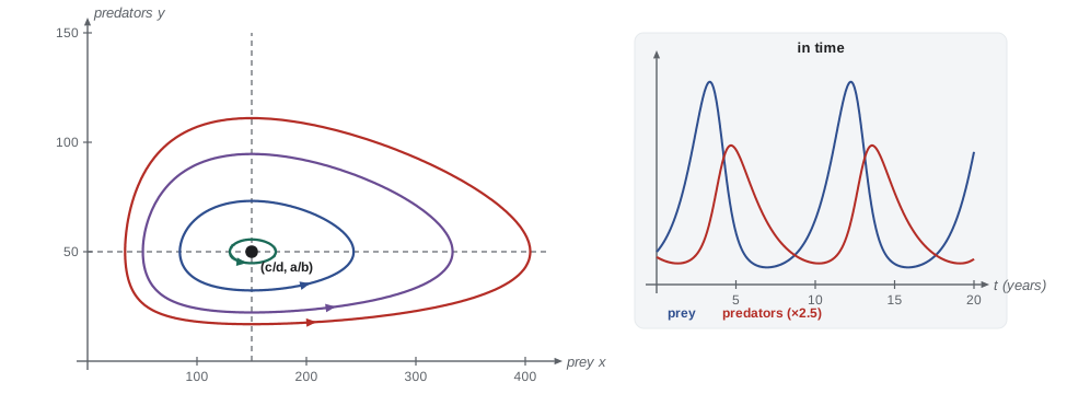
The model explains D'Ancona's observation. Over one cycle the average populations equal the equilibrium values. To see this, write the prey equation as \(\frac{d}{dt}\ln x = a - by\) and integrate over one period \(T\): the left side gives zero, since \(x\) returns to its starting value, so \(\frac{1}{T}\int_0^T y\,dt = \frac{a}{b}\). Likewise the average of \(x\) is \(\frac{c}{d}\). Fishing that removes both species at a rate \(\epsilon\) changes \(a\) to \(a - \epsilon\) and \(c\) to \(c + \epsilon\), so the average prey rises to \(\frac{c + \epsilon}{d}\) and the average predators fall to \(\frac{a - \epsilon}{b}\). Reducing fishing has the opposite effect, raising the proportion of predators, as D'Ancona saw. This result, Volterra's principle, also warns that a pesticide killing both a crop pest and its natural enemy can increase the pest.

Linearization and the Jacobian

Near an equilibrium \((x^*, y^*)\) a nonlinear system behaves approximately like its linearization. Writing \(u = x - x^*\) and \(v = y - y^*\) and expanding \(f\) and \(g\) to first order gives \[\begin{pmatrix} u \\ v \end{pmatrix}^\prime \approx J\begin{pmatrix} u \\ v \end{pmatrix}, \qquad J = \begin{pmatrix} f_x & f_y \\ g_x & g_y \end{pmatrix},\] with the partial derivatives evaluated at the equilibrium. The matrix \(J\) is the Jacobian. The solutions of the linear system are combinations of \(e^{\lambda t}\) where \(\lambda\) runs over the eigenvalues of \(J\), the roots of \(\lambda^2 - \tau\lambda + \Delta = 0\) with \(\tau = \operatorname{tr} J\) and \(\Delta = \det J\).

The eigenvalues classify the equilibrium. If \(\Delta < 0\), the eigenvalues are real with opposite signs and the equilibrium is a saddle, unstable. If \(\Delta > 0\) and \(\tau < 0\), both eigenvalues have negative real part and the equilibrium is stable: a stable node if \(\tau^2 > 4\Delta\) (real eigenvalues) and a stable spiral if \(\tau^2 < 4\Delta\) (complex eigenvalues). If \(\Delta > 0\) and \(\tau > 0\), it is an unstable node or spiral. If \(\Delta > 0\) and \(\tau = 0\), the eigenvalues are purely imaginary and the linearization is a center, with closed orbits.

Theorem 6.1 (Hartman–Grobman, informal). If no eigenvalue of \(J\) has zero real part, then near the equilibrium the phase portrait of the nonlinear system has the same qualitative structure as that of its linearization: saddles stay saddles, stable nodes and spirals stay stable. In the borderline case of a center the nonlinear terms decide, and the equilibrium may be a true center, a weakly stable spiral or a weakly unstable one.

Making the model more realistic

The closed orbits of the Lotka–Volterra model are structurally unstable: an arbitrarily small change to the equations can destroy them. A more realistic model limits prey growth by a carrying capacity \(K\): \[\frac{dx}{dt} = ax\Big(1 - \frac{x}{K}\Big) - bxy, \qquad \frac{dy}{dt} = -cy + dxy.\] Now the \(x\)-nullcline is the sloping line \(y = \frac{a}{b}(1 - \frac{x}{K})\). If \(K > \frac{c}{d}\), it meets the vertical predator nullcline at \(x^* = \frac{c}{d}\), \(y^* = \frac{a}{b}(1 - \frac{c}{dK})\). The Jacobian there has \(\tau = -\frac{ax^*}{K} < 0\) and \(\Delta = bdx^*y^* > 0\), so the coexistence equilibrium is stable, usually a stable spiral. Oscillations now damp out.

Real predator–prey systems sometimes show persistent cycles, the most famous being the ten-year cycle of snowshoe hares and Canada lynx recorded in Hudson's Bay Company fur returns. Models that produce sustained cycles robustly need a further ingredient, such as a predator that becomes satiated at high prey density. These models have a stable limit cycle, an isolated periodic orbit that attracts nearby trajectories, and lesson 12 returns to the question of which model features are needed to match observed behavior.

# Lotka-Volterra with RK4: check the conserved quantity and measure the period
import math
a, b, c, d = 1.0, 0.02, 0.6, 0.004          # per year, per fish per year
def rhs(x, y):
    return a * x - b * x * y, -c * y + d * x * y
def rk4(x, y, h):
    k1 = rhs(x, y)
    k2 = rhs(x + h / 2 * k1[0], y + h / 2 * k1[1])
    k3 = rhs(x + h / 2 * k2[0], y + h / 2 * k2[1])
    k4 = rhs(x + h * k3[0], y + h * k3[1])
    return (x + h / 6 * (k1[0] + 2 * k2[0] + 2 * k3[0] + k4[0]),
            y + h / 6 * (k1[1] + 2 * k2[1] + 2 * k3[1] + k4[1]))
V = lambda x, y: d * x - c * math.log(x) + b * y - a * math.log(y)

x, y, h, t = 100.0, 30.0, 0.001, 0.0
V0, crossings, prev_y = V(x, y), [], y
xs, ys = [], []
while t < 40:
    x, y = rk4(x, y, h); t += h
    xs.append(x); ys.append(y)
    if prev_y < 50 <= y and x > 150:          # upward crossing of y = a/b, right of x* = 150
        crossings.append(t)
    prev_y = y
print("equilibrium (x*, y*) =", (c / d, a / b))
print("drift in V over 40 years:", f"{abs(V(x, y) - V0):.1e}")
print("periods:", [round(t2 - t1, 3) for t1, t2 in zip(crossings, crossings[1:])])
print("mean prey", round(sum(xs) / len(xs), 1), " mean predators", round(sum(ys) / len(ys), 1))
print("linear estimate 2 pi / sqrt(ac) =", round(2 * math.pi / math.sqrt(a * c), 3))

equilibrium (x*, y*) = (150.0, 50.0)
drift in V over 40 years: 3.6e-15
periods: [8.392, 8.391, 8.392, 8.392]
mean prey 153.6  mean predators 50.5
linear estimate 2 pi / sqrt(ac) = 8.112

The output confirms the theory. The quantity \(V\) is conserved to within the accuracy of the integrator, the orbit has a constant period somewhat longer than the linear estimate because the oscillation is large, and the time averages are close to \((150, 50)\), the equilibrium. They are not exactly equal because 40 years is not a whole number of periods.

Competition between species

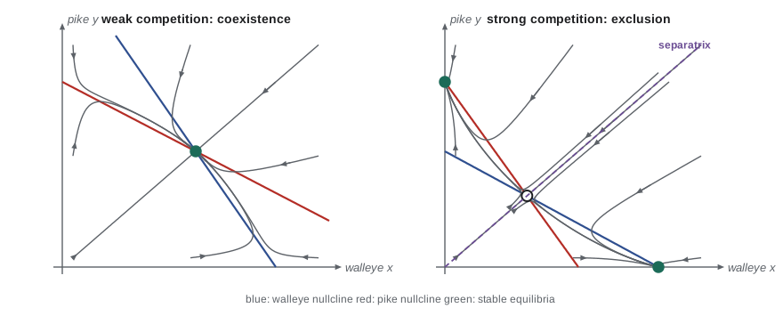
Walleye and northern pike both eat perch. A simple model of two competitors gives each logistic growth, reduced by the other: \[\frac{dx}{dt} = r_1x\Big(1 - \frac{x + \alpha y}{K_1}\Big), \qquad \frac{dy}{dt} = r_2y\Big(1 - \frac{y + \beta x}{K_2}\Big).\] The competition coefficient \(\alpha\) measures the effect of one pike on walleye growth relative to one walleye; \(\beta\) measures the reverse. Besides the origin and the single-species equilibria \((K_1, 0)\) and \((0, K_2)\), there may be a coexistence equilibrium where the straight-line nullclines \(x + \alpha y = K_1\) and \(y + \beta x = K_2\) cross in the positive quadrant.

The outcome depends on how the nullclines are arranged. If \(K_1 > \alpha K_2\) and \(K_2 > \beta K_1\), each species can invade when the other is at its carrying capacity, the nullclines cross, and the coexistence equilibrium is stable: competition between species is weaker than within each species. If \(K_1 > \alpha K_2\) but \(K_2 < \beta K_1\), the nullclines do not cross and species \(x\) wins from every starting point with both present. If \(K_1 < \alpha K_2\) and \(K_2 < \beta K_1\), the nullclines cross at a saddle, and the winner depends on the starting point: whichever species gets established first excludes the other. The tendency of strong competitors to exclude each other is called the competitive exclusion principle.

A checklist for the phase plane

Faced with a new two-dimensional model, work through the same steps: find and sketch the nullclines; mark the direction of motion in each region; find the equilibria; compute the Jacobian at each and classify it by trace and determinant; and finally check numerically, by integrating a few trajectories, that the global picture matches. The local analysis tells what happens near each equilibrium, the nullclines tell how trajectories move between them, and numerical solutions confirm the whole. Lesson 7 applies the checklist to epidemics.