Conservation laws: diffusion and traffic flow

All the models so far have been lumped: one number for the whole lake, the whole city or the whole bus. Many questions depend on position as well as time. How fast does a dissolved pollutant spread along a narrow bay? Where does a traffic jam form behind a red light, and how fast does it move backward? Such questions need distributed models, whose state is a function of position and time and whose equations are partial differential equations. This lesson derives the most important family of such models from a single principle, conservation, and studies two members: the diffusion equation and the traffic flow equation.

Density, flux and conservation

Consider a quantity distributed along a line, such as the mass of a pollutant in a long narrow bay or the number of cars on a highway. Let \(u(x, t)\) be its density, the amount per unit length at position \(x\) and time \(t\), and let \(q(x, t)\) be its flux, the amount crossing position \(x\) per unit time in the positive direction. The amount in an interval \([a, b]\) is \(\int_a^b u\,dx\). If the quantity is neither created nor destroyed, it changes only because of what flows in at \(a\) and out at \(b\): \[\frac{d}{dt}\int_a^b u(x, t)\,dx = q(a, t) - q(b, t) = -\int_a^b \frac{\partial q}{\partial x}\,dx.\]

Since this holds for every interval, and the functions are assumed smooth, the integrands must be equal: \[\frac{\partial u}{\partial t} + \frac{\partial q}{\partial x} = 0.\] This is the conservation law in differential form. If the quantity is produced at a rate \(s(x, t)\) per unit length, for example by a source of pollution or by births in a population, the right side becomes \(s\). The conservation law is exact; it is one equation in two unknowns, \(u\) and \(q\). To close the model we need a constitutive relation expressing the flux in terms of the density. Different constitutive relations give different models, and choosing one is the modeling step.

Diffusion

For a substance spread by random molecular motion, or by small-scale turbulent mixing in water, the flux is from high concentration to low and, to a good approximation, proportional to the concentration gradient. This is Fick's law, \(q = -D\frac{\partial u}{\partial x}\), where \(D > 0\) is the diffusion coefficient, with units of length squared per time. Substituting into the conservation law gives the diffusion equation, also called the heat equation because Fourier's law of heat conduction has the same form: \[\frac{\partial u}{\partial t} = D\frac{\partial^2u}{\partial x^2}.\]

The equation says that \(u\) increases where its graph is concave up and decreases where it is concave down, so peaks are flattened and troughs filled. Dimensional analysis from lesson 2 already tells us the most important fact about it. The only combination of a length \(L\), a time \(t\) and \(D\) that is dimensionless is \(\frac{L^2}{Dt}\). So the distance over which diffusion spreads a substance in time \(t\) is of order \(\sqrt{Dt}\), and the time to spread over a distance \(L\) is of order \(\frac{L^2}{D}\). Doubling the distance quadruples the time. For a dissolved substance in still water, \(D \approx 10^{-9}\) m²/s, and spreading one meter would take about thirty years; in a bay, turbulent mixing gives effective values a million times larger, which is why spills spread over kilometers in days.

The spreading of a spill

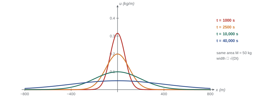
Suppose a mass \(M\) of a dissolved substance is released at \(x = 0\) in a long bay at \(t = 0\). The solution of the diffusion equation with this initial condition is the fundamental solution, \[u(x, t) = \frac{M}{\sqrt{4\pi Dt}}e^{-x^2/(4Dt)}.\] It is a normal density with mean 0 and variance \(2Dt\). Its integral over all \(x\) is \(M\) for every \(t\), as conservation requires; its peak height falls like \(\frac{1}{\sqrt{t}}\), and its width grows like \(\sqrt{t}\). The fundamental solution has the similarity form \(u = \frac{M}{\sqrt{Dt}}F(\frac{x}{\sqrt{Dt}})\), a direct consequence of the scaling argument above.

Separation of variables and decay of modes

On a finite interval \(0 < x < L\) with the ends held at zero, \(u(0, t) = u(L, t) = 0\), the diffusion equation can be solved by separation of variables. Trying \(u = X(x)T(t)\) gives \(\frac{T^\prime}{DT} = \frac{X^{\prime\prime}}{X} = -k^2\), a constant, with solutions \(X = \sin\frac{n\pi x}{L}\) and \(T = e^{-D(n\pi/L)^2t}\) for \(n = 1, 2, \dots\). The general solution is a Fourier sine series \[u(x, t) = \sum_{n=1}^\infty b_n\sin\frac{n\pi x}{L}e^{-D(n\pi/L)^2t},\] with coefficients \(b_n\) determined by the initial profile. Each mode decays at a rate proportional to \(n^2\), so fine-scale wiggles disappear almost instantly and the profile soon looks like the single slowest mode \(n = 1\), which decays on the time scale \(\frac{L^2}{\pi^2D}\). This explains the smoothing effect of diffusion in quantitative terms.

Computing solutions

The diffusion equation is also easy to solve numerically. On a grid \(x_j = j\Delta x\), \(t_m = m\Delta t\), replace the time derivative by a forward difference and the second space derivative by a centered difference: \[\frac{u_j^{m+1} - u_j^m}{\Delta t} = D\frac{u_{j+1}^m - 2u_j^m + u_{j-1}^m}{\Delta x^2}.\] With \(\lambda = \frac{D\Delta t}{\Delta x^2}\), this is \(u_j^{m+1} = \lambda u_{j-1}^m + (1 - 2\lambda)u_j^m + \lambda u_{j+1}^m\), the explicit scheme. It is stable only if \(\lambda \le \frac{1}{2}\). Above this limit, the highest-frequency mode is multiplied at each step by \(1 - 4\lambda < -1\) and grows explosively, with alternating signs, a direct analog of the unstable fixed point with \(F^\prime < -1\) in lesson 4. The restriction \(\Delta t \le \frac{\Delta x^2}{2D}\) means that halving the grid spacing requires quartering the time step, which is why implicit schemes, stable for every time step, are preferred for fine grids.

import math
D, L, nx = 1.0, 1.0, 51                    # scaled units
dx = L / (nx - 1)

def run(lam, t_end=0.05):
    dt = lam * dx * dx / D
    u = [math.sin(math.pi * j * dx) + 0.3 * math.sin(7 * math.pi * j * dx) for j in range(nx)]
    steps = round(t_end / dt)
    for _ in range(steps):
        u = [0.0] + [lam * u[j - 1] + (1 - 2 * lam) * u[j] + lam * u[j + 1] for j in range(1, nx - 1)] + [0.0]
    t = steps * dt
    exact = [math.sin(math.pi * j * dx) * math.exp(-math.pi**2 * D * t)
             + 0.3 * math.sin(7 * math.pi * j * dx) * math.exp(-49 * math.pi**2 * D * t) for j in range(nx)]
    return steps, max(abs(a - b) for a, b in zip(u, exact))

for lam in [0.25, 0.4, 0.5, 0.55, 0.6]:
    steps, err = run(lam)
    print(f"lambda = {lam:4.2f}: {steps:4d} steps, max error {err:.2e}")

lambda = 0.25:  500 steps, max error 4.96e-05
lambda = 0.40:  312 steps, max error 1.39e-04
lambda = 0.50:  250 steps, max error 1.98e-04
lambda = 0.55:  227 steps, max error 1.06e+01
lambda = 0.60:  208 steps, max error 8.90e+12

For \(\lambda \le \frac{1}{2}\) the computed solution matches the exact Fourier solution to a few parts in ten thousand or better. At \(\lambda = 0.55\) the error is already larger than the solution itself, and at 0.6 it is astronomical, even though the time step is only slightly larger: rounding errors excite the highest grid mode, which then grows at every step. Numerical stability is a property of the scheme, not of the equation, and checking it is part of solving any model numerically.

Traffic flow

Now apply the conservation law to cars on a single-lane road, with \(\rho(x, t)\) the density in cars per kilometer and \(q\) the flow in cars per hour. If cars travel at speed \(v\), then \(q = \rho v\). The constitutive assumption of the Lighthill–Whitham–Richards model, proposed in the 1950s, is that drivers adjust their speed to the local density: \(v = V(\rho)\), decreasing from the free speed \(v_{\max}\) on an empty road to zero at the jam density \(\rho_{\max}\), bumper to bumper. The simplest choice, due to Greenshields, is linear: \[V(\rho) = v_{\max}\Big(1 - \frac{\rho}{\rho_{\max}}\Big), \qquad q(\rho) = v_{\max}\rho\Big(1 - \frac{\rho}{\rho_{\max}}\Big).\] The conservation law \(\rho_t + q(\rho)_x = 0\) is now a nonlinear first-order equation.

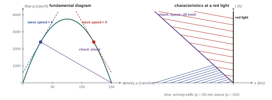
The graph of \(q\) against \(\rho\) is called the fundamental diagram. For the Greenshields law it is a parabola, the same shape as the logistic growth curve, with maximum flow \(q_{\max} = \frac{v_{\max}\rho_{\max}}{4}\) at the critical density \(\frac{\rho_{\max}}{2}\). For \(v_{\max} = 100\) km/h and \(\rho_{\max} = 150\) cars per km, the capacity of the lane is 3750 cars per hour, rather higher than the 2000 or so measured on real highways, which have fundamental diagrams with a sharper peak at lower density. The model's qualitative conclusions do not depend on these details.

Waves and shocks

Writing the conservation law as \(\rho_t + q^\prime(\rho)\rho_x = 0\) shows that density is carried along curves in the \((x, t)\) plane, called characteristics, with speed \[c(\rho) = q^\prime(\rho) = v_{\max}\Big(1 - \frac{2\rho}{\rho_{\max}}\Big).\] Along each characteristic \(\rho\) is constant, so the characteristics are straight lines. This wave speed is not the speed of the cars. In light traffic, \(\rho < \frac{\rho_{\max}}{2}\), waves move forward but slower than the cars. In heavy traffic waves move backward, against the traffic: this is why a disturbance on a busy highway, such as a driver braking, propagates backward as a stop-and-go wave that later drivers meet without ever seeing its cause.

When faster characteristics from behind catch up with slower ones ahead, they cross, and the solution would have several densities at one point. Physically, the density jumps abruptly: a shock forms. Conservation across the jump determines its speed. If the density jumps from \(\rho_1\) behind to \(\rho_2\) ahead, the shock speed is \[s = \frac{q(\rho_2) - q(\rho_1)}{\rho_2 - \rho_1},\] the slope of the chord of the fundamental diagram between the two states. For the Greenshields law this simplifies to \(s = v_{\max}(1 - \frac{\rho_1 + \rho_2}{\rho_{\max}})\).

When the light turns green, the opposite happens: density drops from the jam value to lower values ahead, the characteristics fan out, and the queue dissolves in a rarefaction wave, with the front cars accelerating away and the start-up wave moving backward through the queue at the speed \(c(\rho_{\max}) = -v_{\max}\). The same mathematics describes bus bunching on a larger scale: a bus slowed by a dense cluster of waiting passengers behaves like a moving bottleneck, and the analysis of conservation laws helps transit planners design bus lanes and signal priority.

Other conservation laws

The pattern of this lesson, a conservation law plus a constitutive relation, generates a large part of applied mathematics. Adding diffusion to logistic growth gives Fisher's equation \(u_t = Du_{xx} + ru(1 - u)\), whose traveling waves spread at speed \(2\sqrt{rD}\) and describe the invasion of a new species, such as an invasive fish spreading up a river system. Conservation of mass and momentum for fluids gives the equations of hydraulics and of the atmosphere. Conservation of vehicles, combined with a different constitutive law, gives models of pedestrian crowds. In each case the art of modeling lies in the constitutive relation, which must be justified by mechanism and checked against data.