Fitting models to data: least squares and parameter estimation

A model's parameters must come from somewhere. Some, like the gravitational acceleration, are known from physics; many, like the growth rate of walleye in Larch Lake or the transmission coefficient of this year's influenza, must be estimated from data. This lesson develops the method of least squares, first for models that are linear in their parameters and then for nonlinear models such as the logistic equation, which we fit to the lake's survey counts. Just as important as the estimates are their uncertainties, the diagnostics that show whether the model fits, and the dangers of fitting too much.

Data, residuals and the least squares principle

Suppose a model predicts an output \(f(t; \theta)\) depending on an input \(t\) and a vector of parameters \(\theta\), and we have observations \(y_1, \dots, y_n\) at inputs \(t_1, \dots, t_n\). The residuals \(e_i = y_i - f(t_i; \theta)\) measure the misfit. The least squares estimate \(\hat{\theta}\) minimizes the sum of squared residuals \[S(\theta) = \sum_{i=1}^n \big(y_i - f(t_i; \theta)\big)^2.\]

Why squares? Squaring makes all residuals count positively, penalizes large misfits heavily, and leads to equations that can be solved by linear algebra. There is also a statistical justification: if the observations are the model's predictions plus independent normally distributed errors with constant variance, then the least squares estimate is the maximum likelihood estimate, the parameter value under which the observed data are most probable. When the errors are not like this, other criteria may be better. Counts of fish or cases, for instance, often have errors proportional to their size, and fitting the logarithms of the data is then more appropriate.

Linear least squares

A model is linear in its parameters if \(f(t; \theta) = \theta_1g_1(t) + \cdots + \theta_kg_k(t)\) for known functions \(g_j\). The straight line \(f = \theta_1 + \theta_2t\) and the quadratic \(\theta_1 + \theta_2t + \theta_3t^2\) are examples. Collecting the values \(g_j(t_i)\) into an \(n \times k\) design matrix \(X\), the residual vector is \(y - X\theta\) and \(S(\theta) = \|y - X\theta\|^2\). Setting the gradient to zero gives the normal equations \[X^TX\hat{\theta} = X^Ty.\] If the columns of \(X\) are linearly independent, \(X^TX\) is invertible and \(\hat{\theta} = (X^TX)^{-1}X^Ty\). Geometrically, \(X\hat{\theta}\) is the orthogonal projection of the data vector onto the column space of \(X\), so the residual vector is perpendicular to every column.

Linearizing transformations

Some nonlinear models become linear after a transformation. Exponential growth \(N = N_0e^{\rho t}\) gives \(\ln N = \ln N_0 + \rho t\), a straight line in \(t\) with slope \(\rho\). A power law \(y = Cx^p\) gives \(\ln y = \ln C + p\ln x\). Fitting the transformed model by linear least squares is quick and is a standard first step, for instance in estimating the early growth rate of an epidemic from daily case counts and hence, by lesson 7, its \(R_0\).

Two cautions apply. First, least squares on the transformed scale minimizes a different quantity: relative rather than absolute errors. This is often an advantage for data that span orders of magnitude, but it changes the estimates. Second, the transformation is only valid where the model is. Fitting a straight line to the logarithms of the Larch Lake counts over the first eight years gives a growth rate of about 0.21 per year, well below the true intrinsic rate, because density dependence has already slowed growth by the time the population reaches half its carrying capacity. A linearization should be applied only to the part of the data where its assumptions hold.

Nonlinear least squares

The logistic model \(N(t) = \frac{KN_0}{N_0 + (K - N_0)e^{-rt}}\) is not linear in \(r\), \(K\) and \(N_0\), and no transformation makes it so for all three at once. Minimizing \(S(\theta)\) then requires an iterative method. The Gauss–Newton method linearizes the model around the current guess \(\theta^{(m)}\): \[f(t_i; \theta) \approx f(t_i; \theta^{(m)}) + J_i(\theta - \theta^{(m)}),\] where \(J\) is the \(n \times k\) Jacobian matrix of partial derivatives \(\frac{\partial f(t_i; \theta)}{\partial \theta_j}\). The linearized problem is a linear least squares problem for the step \(\delta = \theta - \theta^{(m)}\), with normal equations \[J^TJ\delta = J^Te,\] where \(e\) is the current residual vector. Solving and updating \(\theta^{(m+1)} = \theta^{(m)} + \delta\), then repeating, usually converges quickly from a reasonable starting guess. The Levenberg–Marquardt method adds a damping term, \((J^TJ + \mu I)\delta = J^Te\), which makes it more reliable from poor starting points, and is the method used by most fitting software.

Good starting values matter, because a nonlinear \(S(\theta)\) can have several local minima. Use the meaning of the parameters: \(K\) is near the level at which the data flatten, \(N_0\) near the first observation, and \(r\) can be estimated from early growth. This is another benefit of mechanistic models: their parameters have interpretations that guide the fitting.

Fitting the Larch Lake survey

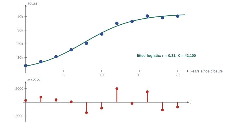
After the fishery was closed in 1998 to let the stock recover, the fisheries office surveyed the adult walleye every two years, with the results below. The counts are estimates from netting surveys, with errors of perhaps 5 to 10 percent.

import numpy as np
t = np.array([0, 2, 4, 6, 8, 10, 12, 14, 16, 18, 20], float)
N = np.array([3900, 7000, 10600, 15700, 20400, 27200, 35100, 36500, 40500, 39200, 40400], float)

def model(p, t):
    r, K, N0 = p
    return K * N0 / (N0 + (K - N0) * np.exp(-r * t))

def jacobian(p, t, h=1e-6):
    J = np.empty((len(t), 3))
    for k in range(3):
        q = np.array(p, float); step = h * max(abs(p[k]), 1.0); q[k] += step
        J[:, k] = (model(q, t) - model(p, t)) / step
    return J

p = np.array([0.2, 35000.0, 5000.0])          # starting guess from the meaning of the parameters
for it in range(8):
    e = N - model(p, t)
    J = jacobian(p, t)
    delta = np.linalg.solve(J.T @ J, J.T @ e)
    p = p + delta
    print(f"iteration {it + 1}: r = {p[0]:.4f}, K = {p[1]:8.0f}, N0 = {p[2]:6.0f}, SSE = {np.sum((N - model(p, t))**2):.4e}")

e = N - model(p, t)
s2 = np.sum(e**2) / (len(t) - 3)              # residual variance with n - k degrees of freedom
cov = s2 * np.linalg.inv(J.T @ J)
se = np.sqrt(np.diag(cov))
for name, val, s in zip(["r", "K", "N0"], p, se):
    print(f"{name:>3} = {val:10.4g}  +/- {1.96 * s:.3g} (95%)")
print("residuals:", " ".join(f"{x:+.0f}" for x in e))
print("correlation of r and N0 estimates:", round(cov[0, 2] / (se[0] * se[2]), 2))

iteration 1: r = 0.3308, K =    37609, N0 =   3349, SSE = 6.1509e+07
iteration 2: r = 0.2932, K =    42094, N0 =   3789, SSE = 1.4090e+07
iteration 3: r = 0.3063, K =    41979, N0 =   3618, SSE = 1.2030e+07
iteration 4: r = 0.3051, K =    42075, N0 =   3637, SSE = 1.2018e+07
iteration 5: r = 0.3053, K =    42069, N0 =   3635, SSE = 1.2018e+07
iteration 6: r = 0.3053, K =    42070, N0 =   3635, SSE = 1.2018e+07
iteration 7: r = 0.3053, K =    42070, N0 =   3635, SSE = 1.2018e+07
iteration 8: r = 0.3053, K =    42070, N0 =   3635, SSE = 1.2018e+07
  r =     0.3053  +/- 0.0446 (95%)
  K =  4.207e+04  +/- 2.08e+03 (95%)
 N0 =       3635  +/- 1.04e+03 (95%)
residuals: +265 +760 +384 +80 -1517 -859 +2005 -170 +1546 -1119 -700
correlation of r and N0 estimates: -0.91

The iteration converges in a few steps. The estimates are \(r \approx 0.31\) per year with a 95% interval of about \(\pm 0.045\), and \(K \approx 42{,}000\) with an interval of about \(\pm 2100\). These intervals come from the standard linearization: near the minimum, the covariance matrix of the estimates is approximately \(s^2(J^TJ)^{-1}\), where \(s^2 = \frac{S(\hat{\theta})}{n - k}\) estimates the error variance with \(n - k\) degrees of freedom. The estimates of \(r\) and \(N_0\) are strongly negatively correlated: a smaller starting population with a faster growth rate fits nearly as well as a larger one with a slower rate. Such correlations are common, and they mean that the individual intervals understate how well some combinations of parameters are determined and overstate how well others are.

Is the fit any good?

A small residual sum of squares is not enough. The key diagnostic is the residual plot. If the model is adequate, residuals should look like random noise: scattered above and below zero with no trend, no curvature and no change in spread. A run of positive residuals followed by a run of negative ones indicates systematic misfit, meaning the model's shape is wrong. Residuals whose spread grows with the fitted value suggest that errors are proportional and the data should be fitted on a log scale. For Larch Lake the residuals alternate irregularly in sign with no evident pattern, so the logistic model is consistent with the data, though eleven points cannot rule out alternatives such as the Gompertz model.

The fitted parameters also answer the management question of lesson 5. With \(\hat{r} = 0.31\) and \(\hat{K} = 42{,}000\), the estimated MSY is \(\frac{\hat{r}\hat{K}}{4} \approx 3200\) fish per year. But propagating the uncertainty, including the correlation between the two estimates, the lower end of a 95% range for \(rK\) is about 11,350 fish per year, giving an MSY near 2840. Because lesson 5 showed that overestimating MSY is dangerous, a precautionary policy would base the catch on the lower value, or better, on a constant effort.

Identifiability

A parameter is identifiable from given data if different values of it produce detectably different predictions. If the Larch Lake surveys had stopped after six years, while the population was still growing almost exponentially, the data would determine \(r\) reasonably well but say almost nothing about \(K\): many carrying capacities fit the early curve equally well. The matrix \(J^TJ\) would be nearly singular, and the standard error of \(K\) enormous. Before fitting, it is worth asking which parameters the data can possibly determine, and before collecting data, which measurements would best determine the parameters that matter for the decision. In the influenza model, early case counts determine the growth rate \(\gamma(R_0 - 1)\) but not \(R_0\) and \(\gamma\) separately, which is why estimates of the infectious period from clinical studies are needed as well.

Overfitting and model selection

Adding parameters always reduces the residual sum of squares, since the extra flexibility can only help the fit. A polynomial of degree 10 passes exactly through the 11 survey points, with zero residuals, but wiggles wildly between them and predicts nonsense beyond them. This is overfitting: the model has fitted the noise as well as the signal. Several defenses are available. The simplest is to compare models on data not used for fitting, by holding back some observations or by cross-validation, in which each point is predicted from a fit to the others. Another is to penalize the number of parameters. The Akaike information criterion for least squares fits with normal errors is \[\mathrm{AIC} = n\ln\frac{S(\hat{\theta})}{n} + 2k,\] and among candidate models the one with the smallest AIC is preferred. A mechanistic model with three interpretable parameters that fits nearly as well as a twelve-parameter polynomial is almost always the better choice, because its structure encodes real knowledge.