Discrete-time models: difference equations and cobwebs

Many systems change in steps rather than continuously. Walleye spawn once a year in spring, a savings account is credited monthly, and a bus passes one stop after another. A discrete-time model describes the state after each step as a function of the state before it. This lesson develops the basic tools: linear difference equations, fixed points and their stability, cobweb diagrams, and the remarkable behavior of simple nonlinear maps, which can oscillate and even become chaotic. We finish by turning the bus bunching argument of lesson 1 into a difference equation and using it to design a holding strategy.

First-order difference equations

A first-order difference equation, or map, has the form \[x_{t+1} = F(x_t), \qquad t = 0, 1, 2, \dots,\] where \(x_t\) is the state at step \(t\) and \(F\) is a given function. Starting from an initial value \(x_0\), the equation determines \(x_1 = F(x_0)\), \(x_2 = F(x_1)\), and so on. The sequence \(x_0, x_1, x_2, \dots\) is called an orbit. Unlike a differential equation, a difference equation can always be solved numerically exactly, simply by iterating, so the question is never whether a solution exists but how it behaves.

The simplest case is linear growth, \(x_{t+1} = \lambda x_t\), with solution \(x_t = \lambda^tx_0\). If \(|\lambda| < 1\) the orbit tends to 0; if \(|\lambda| > 1\) it grows without bound; if \(\lambda < 0\) it alternates in sign. Adding a constant input gives the affine equation \(x_{t+1} = \lambda x_t + c\). Its fixed point, the value that does not change, solves \(x^* = \lambda x^* + c\), so \(x^* = \frac{c}{1 - \lambda}\) when \(\lambda \ne 1\). Writing \(y_t = x_t - x^*\) gives \(y_{t+1} = \lambda y_t\), so \[x_t = x^* + \lambda^t(x_0 - x^*).\]

Fixed points and linear stability

For a nonlinear map, a fixed point \(x^*\) satisfies \(F(x^*) = x^*\). To decide whether nearby orbits approach it, linearize. Write \(x_t = x^* + y_t\) with \(y_t\) small. Then by Taylor's theorem \[x^* + y_{t+1} = F(x^* + y_t) = F(x^*) + F^\prime(x^*)y_t + O(y_t^2),\] so to first order \(y_{t+1} \approx F^\prime(x^*)y_t\). The perturbation behaves like the linear equation with \(\lambda = F^\prime(x^*)\).

Theorem 4.1 (linear stability of fixed points). Let \(F\) be continuously differentiable near a fixed point \(x^*\). If \(|F^\prime(x^*)| < 1\), then \(x^*\) is locally asymptotically stable: orbits starting close enough to \(x^*\) converge to it. If \(|F^\prime(x^*)| > 1\), then \(x^*\) is unstable. If \(0 < F^\prime(x^*) < 1\) the approach is monotone, and if \(-1 < F^\prime(x^*) < 0\) it is oscillatory, with the orbit jumping from one side of \(x^*\) to the other.

Proof sketch for the stable case. Choose \(k\) with \(|F^\prime(x^*)| < k < 1\). By continuity of \(F^\prime\) there is \(\delta > 0\) with \(|F^\prime(x)| \le k\) for \(|x - x^*| \le \delta\). By the mean value theorem, if \(|x_t - x^*| \le \delta\) then \(|x_{t+1} - x^*| = |F(x_t) - F(x^*)| \le k|x_t - x^*|\), which is again at most \(\delta\). By induction \(|x_t - x^*| \le k^t|x_0 - x^*| \to 0\). This is the same contraction argument that proves the Banach fixed point theorem. \(\square\)

When \(|F^\prime(x^*)| = 1\) the linear test is inconclusive and higher-order terms decide. Such borderline cases mark the boundaries between different kinds of behavior and are called bifurcation points.

Cobweb diagrams

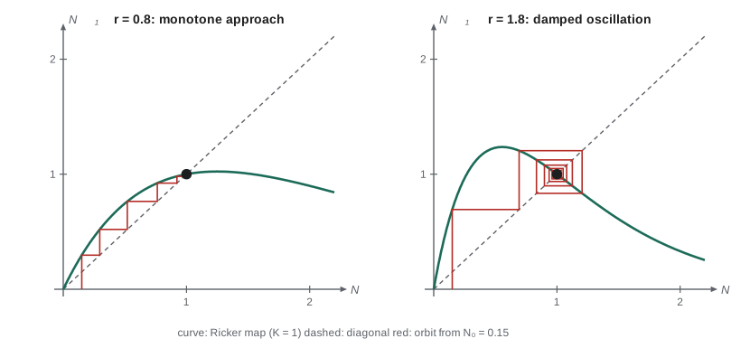
A cobweb diagram shows the orbit of a one-dimensional map geometrically. Plot the graph \(y = F(x)\) together with the diagonal \(y = x\); fixed points are where they cross. From \((x_0, x_0)\) on the diagonal, move vertically to the graph, reaching \((x_0, x_1)\), then horizontally back to the diagonal at \((x_1, x_1)\), then vertically to \((x_1, x_2)\), and so on. The staircase or spiral that results shows at a glance whether the orbit converges, oscillates or wanders.

Near a fixed point the slope of the graph decides the shape. A slope between 0 and 1 gives a staircase converging monotonically; a slope between \(-1\) and 0 gives a spiral converging with oscillation; a slope below \(-1\) gives a spiral moving outward. This is Theorem 4.1 in pictures, and drawing a cobweb is the fastest way to build intuition about an unfamiliar map.

Spawning stock and recruitment

Walleye in Larch Lake spawn each spring, and the number of young fish that survive to join the adult population, called recruitment, depends on the number of spawners. When spawners are few, recruitment rises in proportion; when they are many, young fish compete for food and are eaten by adults, so recruitment levels off or even declines. Two classical models capture these cases. The Beverton–Holt model \[N_{t+1} = \frac{RN_t}{1 + \frac{(R - 1)N_t}{K}}\] has recruitment that saturates, while the Ricker model \[N_{t+1} = N_te^{r(1 - N_t/K)}\] has recruitment that falls at high density. In both, \(K\) is a positive fixed point, the carrying capacity.

For the Beverton–Holt model, \(F^\prime(K) = \frac{1}{R}\), which lies between 0 and 1 whenever \(R > 1\). Its positive equilibrium is always stable, and the approach is always monotone. The two models agree near equilibrium when \(r\) is small but behave very differently for large \(r\), so the choice between them matters. Fisheries biologists decide between them from stock and recruitment data, which for many species show a clear decline at high spawner numbers.

Beyond stability: cycles and chaos

What happens to the Ricker model when \(r > 2\)? The fixed point is unstable, but orbits remain bounded, since \(F(N) \le \frac{K}{r}e^{r - 1}\) for all \(N\). Just above \(r = 2\) the orbit settles into a cycle of period 2, alternating between a high and a low value. Such a cycle consists of fixed points of the second iterate \(F^2 = F \circ F\), and its stability is decided by \(|(F^2)^\prime| = |F^\prime(p)F^\prime(q)| < 1\), where \(p\) and \(q\) are the two values. As \(r\) increases further the 2-cycle loses stability to a 4-cycle, then an 8-cycle, in a cascade of period doublings that accumulates near \(r \approx 2.69\). Beyond that, for most values of \(r\), the orbit never settles: it is chaotic.

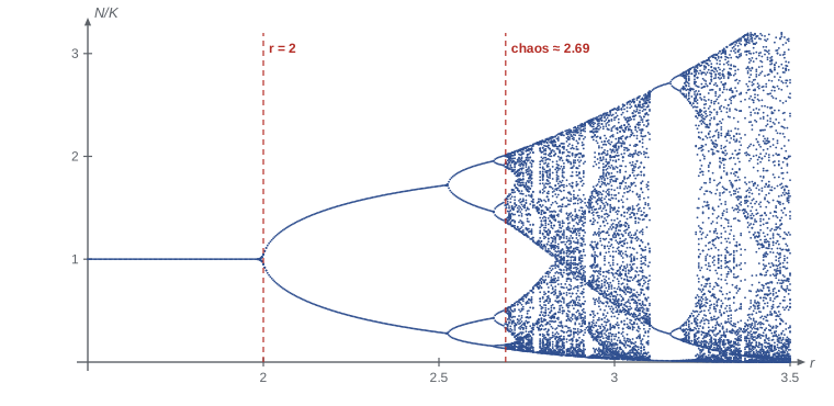
Chaos means sensitive dependence on initial conditions: two orbits that start very close separate exponentially fast, so long-range prediction is impossible even though the model is completely deterministic. Robert May drew attention to this in 1976, pointing out that the simplest nonlinear population models could produce apparently random fluctuations without any external noise. Whether real populations are chaotic is still debated; but the discovery changed how ecologists interpret fluctuating data, since irregular counts need not mean that the environment is irregular.

import math

def ricker(N, r, K=1.0):
    return N * math.exp(r * (1 - N / K))

for r in [0.8, 1.8, 2.3, 2.6, 3.0]:
    N = 0.2
    for _ in range(1000):          # discard the transient
        N = ricker(N, r)
    tail = []
    for _ in range(8):
        N = ricker(N, r); tail.append(N)
    print(f"r = {r}:  " + "  ".join(f"{x:.3f}" for x in tail))

# sensitive dependence: two orbits starting 1e-9 apart when r = 3.0
a, b = 0.3, 0.3 + 1e-9
for t in range(1, 41):
    a, b = ricker(a, 3.0), ricker(b, 3.0)
    if t % 8 == 0:
        print(f"step {t:2d}: difference {abs(a - b):.2e}")

r = 0.8:  1.000  1.000  1.000  1.000  1.000  1.000  1.000  1.000
r = 1.8:  1.000  1.000  1.000  1.000  1.000  1.000  1.000  1.000
r = 2.3:  1.592  0.408  1.592  0.408  1.592  0.408  1.592  0.408
r = 2.6:  1.523  0.391  1.905  0.181  1.523  0.391  1.905  0.181
r = 3.0:  2.331  0.043  0.760  1.562  0.289  2.440  0.032  0.592
step  8: difference 1.52e-08
step 16: difference 1.02e-07
step 24: difference 6.68e-06
step 32: difference 5.11e-04
step 40: difference 3.10e-02

The output shows each regime. For \(r = 0.8\) and \(1.8\) the orbit sits at the equilibrium \(N = K = 1\). For \(r = 2.3\) it alternates between two values, for \(r = 2.6\) it cycles through four, and for \(r = 3.0\) it shows no pattern. The second part shows a difference of one part in a billion growing to the size of the population itself within a few dozen steps.

Bus bunching as a difference equation

Return to Route 9. Let \(d_s\) be the delay of a bus, in minutes behind schedule, as it leaves stop \(s\), and suppose the bus ahead is on time. As computed in lesson 1, the bus finds \(\lambda(H + d_s)\) passengers at the next stop, where \(H\) is the scheduled headway, so its dwell time exceeds the scheduled \(\beta H\) by \(\beta d_s\), where \(\beta = b\lambda\). Thus \[d_{s+1} = (1 + \beta)d_s,\] a linear map with multiplier \(1 + \beta > 1\). The on-time state \(d = 0\) is an unstable fixed point, and any delay grows geometrically, as \(d_s = (1 + \beta)^sd_0\).

A holding strategy changes the map. Suppose that at every stop where a bus is early, or at a timing point, a controller removes a fraction \(\alpha\) of the current deviation, by holding early buses and by telling late buses to skip the layover. The map becomes \(d_{s+1} = (1 + \beta)(1 - \alpha)d_s\), which is stable when \((1 + \beta)(1 - \alpha) < 1\), that is \(\alpha > \frac{\beta}{1 + \beta}\). With \(\beta = 0.1\), correcting just over 9% of the deviation at each stop is enough to stop bunching from growing. Real transit agencies implement this through schedules with slack at timing points, and more recently through headway-based control using real-time vehicle locations.

Higher-order equations and systems

Some discrete models involve more than one past value, such as \(x_{t+1} = ax_t + bx_{t-1}\). Trying \(x_t = \mu^t\) gives the characteristic equation \(\mu^2 = a\mu + b\), and the general solution is a combination of \(\mu_1^t\) and \(\mu_2^t\). The solution decays to zero exactly when both roots satisfy \(|\mu| < 1\). Equivalently, writing \(u_t = (x_t, x_{t-1})\) turns the equation into a first-order system \(u_{t+1} = Au_t\) whose eigenvalues are the roots. Age-structured population models, with separate counts of juveniles and adults, are systems of exactly this kind. Their long-run growth rate is the dominant eigenvalue of a matrix called the Leslie matrix, and lesson 9 meets a closely related matrix in Markov chains.