Surveys for design

Every engineering project starts on paper and ends on the ground, and the surveyor is involved at both ends. Before an engineer can design a bridge, a road or a pump station, someone has to measure what is already there: the shape of the ground, the location of buildings, fences, pipes and wires, the water levels, and the legal boundaries that limit where the work can go. After the design is finished, someone has to put it back on the ground with stakes, marks and machine guidance. This course follows Coulee Geomatics through both halves of that work on one large job, and this first lesson covers the first half: the surveys that feed design.

The job is the irrigation district's headworks rehabilitation near Great Falls. The 1957 gate structure on the Sun River diversion is being rebuilt, a new pump station will lift water to a high-level lateral, a siphon will carry a pipeline under the river, and the state is realigning the highway that crosses the main canal, with a new bridge over the canal. Ruth Albrecht leads the survey work for the firm; Ines Dahl runs the field crews; Leah Tran handles research and drafting; Theo Martel does the computations and the data management; Grant Okonkwo leads a crew; and Mira Sandvik, who worked with the firm on the port survey in GEOM-360, joins for the river crossing.

What design needs from a survey

A design survey answers a set of questions that the designers will ask, and the best way to plan one is to ask those questions first. Where exactly are the existing features that the design must connect to, avoid or remove? What is the shape of the ground, closely enough to compute earthwork and drainage? Where are the buried utilities? Where are the property lines and the rights of way, and who owns what? What are the water levels in the river and the canal at different seasons? And what control will the construction surveys use later, so that the design and the stakeout share one coordinate system?

The answers come in several layers. The first is the control network: a set of well-monumented points with known coordinates and heights, spread over the site, from which everything else is measured. The second is the topographic survey: the ground surface, the edges of pavement, ditches, banks, structures and anything else that will appear on the drawings. The third is the utility survey: what is buried, where, and how deep. The fourth is the legal survey: boundaries, rights of way and easements, which GEOM-410 covered. The fifth is a set of special surveys for particular needs, such as a hydrographic survey of the river bed at the siphon crossing (GEOM-360) or a lidar scan of the old gate structure (GEOM-350). The design survey brings all of these into one model that the engineers can trust.

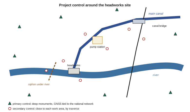
Control first

Control is the skeleton of the project. Everything that follows, from the topographic points to the last as-built shot, hangs on it, and an error in the control spreads into every product. Ruth's rule is that control must be better than anything that depends on it, by a comfortable margin, and must outlast the job. For this project the primary control is eight monuments around the site, set as deep concrete-filled pipes or rods driven to refusal, with brass caps, placed where construction will not disturb them: beyond the work limits, away from haul roads, and with clear sky for GNSS. Each primary monument is observed by static GNSS sessions tied to the national network, and the whole set is adjusted together by least squares, as in GEOM-220.

Secondary control is denser and closer to the work. Around the pump station, the bridge and the siphon shafts, the crew sets points that a total station can see from typical setup positions, measured by traverse from the primary monuments, and adjusted with them. The secondary points will be destroyed one by one as the work proceeds, so the crew sets more than it needs and checks them often. Vertical control is a line of benchmarks run by differential leveling from the primary monuments that have the best height information, closed in loops, and adjusted. GNSS heights are good to a couple of centimeters; leveling is good to a millimeter or two over the site, and the pump station's floors and the siphon's grades need the better figure.

In Montana, the control is tied to the National Spatial Reference System through nearby NGS marks and continuously operating reference stations, with coordinates in NAD83 on the Montana State Plane system and heights in NAVD 88, as GEOM-230 and GEOM-340 described. The Montana Department of Transportation's survey manual sets out its own requirements for control on highway projects, and the district's engineer specifies the coordinate system, the units and the accuracies in the survey scope. Ruth asks for the scope in writing before the first monument is set, because a change of datum halfway through a project, or a mix-up between the international foot and the old survey foot, is expensive and error-prone.

Grid, ground and the project datum

Engineers design in a world where a 100 ft dimension on a drawing is 100 ft on the ground. Map projections do not quite cooperate. As GEOM-340 showed, a distance computed from grid coordinates differs from the same distance measured on the ground by the grid scale factor, and the ground at the site is above the ellipsoid, so a second factor, the elevation factor, also applies. Their product is the combined factor. If the design is drawn in grid coordinates and the crew stakes the grid distances on the ground without correction, every staked dimension will be wrong by the combined factor.

import math
# Project control for the headworks and bridge site: from grid to ground and back
R = 6371000.0            # mean radius of the Earth, m
sites = {
    'ca': dict(k_grid=0.999993, H=900.0, N=-15.0, u='m', f=1.0, dists=(100.0, 500.0, 2000.0)),
    'us': dict(k_grid=0.999455, H=1010.0, N=-15.0, u='ft', f=0.3048, dists=(300.0, 1500.0, 6000.0)),
}
site = sites['us']
h = site['H'] + site['N']                 # ellipsoid height
k_elev = R / (R + h)                      # elevation (height) factor
k_comb = site['k_grid'] * k_elev          # combined factor: grid = ground x k_comb
print(f"grid scale {site['k_grid']:.6f}  elevation factor {k_elev:.6f}  combined {k_comb:.6f}")
u = site['u']                             # heights above are in m; distances in the local unit
for ground in site['dists']:
    grid = ground * k_comb
    print(f"ground {ground:8.3f} {u} -> grid {grid:9.4f} {u}  (difference {ground-grid:.4f} {u} = {(ground-grid)*site['f']*1000:.0f} mm)")
ppm = (1 - k_comb) * 1e6
L = site['dists'][1]
print(f"distortion {ppm:.0f} ppm; a {L:.0f} {u} stakeout from grid coordinates would be short by {ppm*L*site['f']/1000:.0f} mm")

# A project (low-distortion) datum: scale grid coordinates about a project origin so grid = ground at site height
E0, N0 = 1000.000, 5000.000               # (coordinate units as the project uses)
def to_project(E, N): return (E0 + (E - E0) / k_comb, N0 + (N - N0) / k_comb)
E, N = to_project(1500.000, 5300.000)
print(f"grid point (1500.000, 5300.000) -> project ({E:.3f}, {N:.3f})")

grid scale 0.999455  elevation factor 0.999844  combined 0.999299
ground  300.000 ft -> grid  299.7897 ft  (difference 0.2103 ft = 64 mm)
ground 1500.000 ft -> grid 1498.9484 ft  (difference 1.0516 ft = 321 mm)
ground 6000.000 ft -> grid 5995.7936 ft  (difference 4.2064 ft = 1282 mm)
distortion 701 ppm; a 1500 ft stakeout from grid coordinates would be short by 321 mm
grid point (1500.000, 5300.000) -> project (1500.351, 5300.210)

At the headworks the state plane grid scale factor is 0.999455, because the site lies between the standard parallels of the single Montana zone, and the ground is about 995 m above the ellipsoid, so the combined factor is 0.999299. That is 701 parts per million: a 1,500 ft distance on the ground is about 1.05 ft shorter on the grid. Staking a highway from grid distances without correction would put stakes visibly out of place, and even the 79 ft pump station would be about 0.06 ft short. The project datum in the code scales the grid coordinates about an origin near the middle of the site, so that a distance computed from project coordinates equals the ground distance at the site height. The cost is that project coordinates are no longer true state plane coordinates, so every file must say clearly which system it is in. Many agencies, including several state transportation departments, now use low-distortion projections designed for a region, which achieve the same effect with a properly defined projection rather than an ad hoc scale.

There are three common ways to handle the problem, and a project must choose one and stick to it. The first is to design and stake in grid coordinates and apply the combined factor to every distance in the field, which the data collector can do automatically. The second is to create a project datum, as in the code, so that grid equals ground on the site. The third is to use a low-distortion projection, a real map projection with parameters chosen so that the distortion is small at the site's height. Theo's job is to write down which method the project uses, with the parameters, in a control report that every designer and crew lead receives. The most common cause of a staking error on a large project is not a bad measurement; it is two people working in two coordinate systems without knowing it.

The topographic survey

The topographic survey gives the designers a surface they can design on, and the designers must say what they need before the crew goes out. For earthwork on the highway approaches, a digital terrain model good to a few centimeters vertically is enough, and a lidar or photogrammetric survey from the air or a drone, checked on the ground, is efficient (GEOM-310 and GEOM-350). For the pump station site, where the floor elevations and the connections to existing pipes must be exact, ground survey by total station or GNSS is better, with breaklines along every change of slope: the top and toe of banks, the edges of the canal lining, the crown and edges of the road, the lips of ditches. A terrain model built from random points without breaklines will round off every sharp edge and give the designers a canal with soft shoulders that does not exist.

Point density follows the ground. On a smooth field, points every 10 to 20 ft x 3 may be enough; on the rough bank of the coulee, points every couple of meters and breaklines at every change are needed. Grant's crew codes every point as it is collected, so that the software can draw lines and build the surface automatically, and Theo reviews the surface the same day by looking at contours and three-dimensional views. A contour that crosses a breakline, or a sudden spike, shows a coding error or a bad shot, and it is far cheaper to fix it while the crew is still on site.

The survey also picks up everything the designers might need to connect to or avoid: the existing gate structure, pipes, culverts, fences, power poles and guy wires, trees, wells, signs, and the edges of the existing highway. For the old headworks, the lidar scan from GEOM-350 already exists, and Theo checks it against a dozen total-station shots on hard features before the designers use it. A scan that is internally beautiful but shifted by five centimeters as a whole is worse than useless if no one knows about the shift.

Utilities and other hidden things

Buried utilities are the most common source of trouble on construction sites and the most dangerous. Before any digging, Montana 811 must be notified, as HSE-230 described for Oklahoma's system, and the owners locate and mark their lines. For design, though, locates are not enough: the designers need the depth and position of each line at the points where the new work will cross it. The utility survey combines records from the owners, surface features such as valve boxes, manholes and markers, electromagnetic and ground-penetrating radar sweeps, and finally test holes dug by vacuum excavation at critical crossings to expose the line and measure its top. The survey records which information came from which source, because a line drawn from a 1970s record is not the same as a line exposed and measured last week.

Engineers often describe this with quality levels, from D (information from records or memory only) through C (surface features surveyed and correlated with records) and B (lines detected by geophysical methods and marked) to A (lines exposed and measured). The idea comes from the American Society of Civil Engineers' standard for subsurface utility engineering, and a newer standard extends it to the recording of utilities exposed during construction; Canadian practice uses a similar scheme through a CSA standard on mapping underground utility infrastructure. For this project, the highway crossing of a high-pressure gas line and the pump station's connection to a buried power cable are both quality level A; most other lines are B or C.

Water, banks and seasons

The river crossing and the headworks also need water information: water levels on the day of each survey, the levels the district records at its gauge, the river bed from a hydrographic survey, and the banks from lidar or ground survey. Mira's crew will survey the river bed at the siphon crossing by single-beam echo sounder from a small boat at low water, tied to the same control, as GEOM-360 described. The water surface is surveyed at several points on each survey day so that the designers can relate the bed to the water and to the flood levels the engineers have computed. A crossing designed on a bed surveyed at high water, without knowing it, may put the siphon too shallow.

Delivering the design survey

The products of a design survey are a control report, a base plan or model, a terrain surface, a utility report, a boundary and right-of-way plan, and supporting files. The control report lists every control point with its coordinates, heights, accuracy, monument description, and the datum and projection details, including the combined factor or project datum used. The base model, delivered in the designers' software format, shows every feature with its code and layer. The surface is delivered as a terrain model with breaklines. Everything carries metadata: who collected it, when, with what equipment, and how accurate it is. Theo's last task is a checklist that compares the delivered model with the original list of design needs, item by item.

A design survey is never finished in the sense that nothing will change. Construction may not start for a year, and by then a farmer may have moved a fence, the highway department may have added a sign, and the river will have moved some gravel. Ruth's practice is to re-check the control and walk the site before construction staking starts, and to update the base model for anything that has changed near the work.