
GCP-220 · Lesson 3 of 12 · 21 min
Exploring and profiling data
▶ Video coming soon A video version of this lesson is on the way.
On Tuesday, October 13, Mateo brings a question to the session. The store systems team has sent the first week of till exports to the landing bucket, gs://bl-data-landing/pos/, and he wants to load them. Ravi asks him to wait. "What is in the files?" he asks. Mateo knows the columns from the data contract, but he does not know how many rows are empty, whether any store sends negative quantities, or whether the timestamps really are local time. Finding out is called profiling, and it comes before cleaning and loading.
What profiling is for
Data profiling is the systematic inspection of a dataset to learn its shape and its problems. It answers practical questions: how many rows are there, which columns are often empty, how many distinct values does each column have, what are the minimum and maximum, which values are most common, and do the values follow the expected pattern? The answers tell you which cleaning rules you need, which assumptions in the data contract are wrong, and which quality checks to add later.
Profiling is also how you avoid surprises in front of an audience. Ravi remembers a sales dashboard at his previous job that showed a spectacular week, which turned out to be one store's till sending every transaction twice. A five-minute profile would have shown that one store's row count had doubled overnight.
| Profile measure | Question it answers | Example finding |
|---|---|---|
| Row count (per file, per day, per store) | Did everything arrive, and is the volume normal? | Store 027 sent 0 rows on Sunday |
| Null or empty rate per column | Which fields are missing, and how often? | tender is empty on 3 in every 100 rows |
| Distinct count | Is a supposed identifier unique? How many categories are there? | txn_id is not unique: refunds reuse the sale's id |
| Minimum and maximum | Are values within a sensible range? | qty ranges from -4 to 60 |
| Most frequent values | Are there placeholders or default values? | unit_price of 0.00 appears 212 times |
| Pattern or format | Do values follow the expected shape? | Some sku values are lowercase |
| Distribution | Are there outliers or a skew? | Most baskets are under 200 dollars; a few exceed 5,000 |
Exploring files before loading them
The files are still in Cloud Storage, and there are three ways to look at them without loading them into a permanent table. The simplest is to download a sample and open it, which works for small files but does not scale. The second is to create an external table in BigQuery that points at the files: BigQuery reads the files where they sit each time it is queried, so Mateo can run SQL over them straight away. The third is to load the files into a scratch dataset with a table expiration, so the tables delete themselves after a few days.
bq mk --external_table_definition=@CSV=gs://bl-data-landing/pos/2026/10/*.csv \
  bl-data-prod:scratch.pos_explore

# Or, with an explicit schema file:
bq mk --external_table_definition=pos_sales_schema.json@CSV=gs://bl-data-landing/pos/2026/10/*.csv \
  bl-data-prod:scratch.pos_explore
External tables are excellent for exploration but slower and more limited than native tables for regular use: BigQuery cannot cache results from them in the same way, and some table features are not available. That is a theme of lesson 6. For now, the external table lets Mateo run profiling queries over seven days of files in seconds.
Profiling with SQL
A handful of SQL patterns cover most profiling. Ravi encourages Mateo to keep them in a saved query he can reuse for every new feed.
SELECT
  COUNT(*)                                   AS row_count,
  COUNT(DISTINCT store_id)                   AS stores,
  COUNTIF(tender IS NULL OR tender = '')     AS tender_missing,
  COUNTIF(qty < 0)                           AS negative_qty,
  COUNTIF(unit_price = 0)                    AS zero_price,
  MIN(unit_price) AS min_price, MAX(unit_price) AS max_price,
  APPROX_COUNT_DISTINCT(txn_id)              AS approx_txn_ids,
  APPROX_QUANTILES(qty * unit_price, 4)      AS line_value_quartiles
FROM `bl-data-prod.scratch.pos_explore`;
Two functions in that query are worth knowing for the exam. APPROX_COUNT_DISTINCT gives a close estimate of the number of distinct values much more cheaply than an exact COUNT(DISTINCT) on very large tables. APPROX_QUANTILES returns values that split the data into equal parts; asking for 4 gives the minimum, the three quartiles and the maximum, which is a quick way to see the spread and spot outliers. For row counts per store per day, a GROUP BY on store_id and the date does the job, and sorting by the count shows the stores that sent nothing or twice as much as usual.
Profiling in the console and in notebooks
BigQuery and its related tools can profile data without hand-written SQL. Mateo tries each one on the week of till data.
| Tool | What it does | Cost and limits to know |
|---|---|---|
| Table preview | Shows the first rows of a native table | Free; does not run a query; not available for external tables or views |
| Schema and details tabs | Show column types, row count and size | Free |
| Data profile scans (Dataplex Universal Catalog) | Compute null rates, distinct counts, ranges and top values for each column, on a schedule if wanted | Billed for the processing used; can scan a sample to save cost |
| Data insights (Gemini in BigQuery) | Suggests questions and queries about a table based on its profile | Needs Gemini in BigQuery to be set up; suggestions must still be checked |
| BigQuery Studio notebooks or Colab Enterprise | Python notebooks next to the data, with pandas and charts | Notebook runtime is billed while it runs |
A data profile scan is especially useful because it can run on a schedule and keep a history, so the team can see when a column's null rate creeps up over weeks. Data profiling and data quality scans belong to Dataplex, which Google now presents as Dataplex Universal Catalog. Lesson 10 uses its sibling, the data quality scan, to turn profile findings into rules that fail when data goes wrong.
Profiling queries cost money like any other query, because BigQuery's on-demand pricing charges for the bytes a query reads. Before running a query on a large table, Mateo checks the estimate the query editor shows, or runs it as a dry run, which reports the bytes that would be processed without running it. On the warehouse history, a profile that reads every column of 1.2 TB would be far more expensive than one that reads only the five columns he is interested in. Because BigQuery stores data by column, selecting fewer columns is the main way to reduce cost. A LIMIT clause, by contrast, does not reduce the bytes read on a normal table.
bq query --use_legacy_sql=false --dry_run \
  'SELECT store_id, qty, unit_price FROM `bl-data-prod.raw.history_sales`'
# Query successfully validated. This query will process 61,442,108,416 bytes of data.
A quick profile in Python
Sometimes it is quicker to profile a sample in a notebook. Mateo takes forty rows from one store's file and writes a small profile to see what kinds of problems to look for in the full data.
import csv, io
from collections import Counter

sample = """store_id,txn_id,txn_ts,sku,qty,unit_price,discount,tender
012,T5501,2026-10-07 09:14:03,TNT-2P-GRN,1,289.00,,CARD
012,T5502,2026-10-07 09:20:41,stk-al-08,2,14.50,,CASH
012,T5503,2026-10-07 09:31:10,SLP-BAG-0C,1,159.99,15.00,CARD
012,T5503,2026-10-07 09:31:10,SLP-BAG-0C,1,159.99,15.00,CARD
012,T5504,2026-10-07 10:02:55,HDL-LMP-01,1,0.00,,
012,T5505,2026-10-07 10:15:20,TNT-2P-GRN,-1,289.00,,CARD
012,T5506,2026-10-07 10:40:09,BTL-1L-BLU,3,19.95,,card
"""
rows = list(csv.DictReader(io.StringIO(sample)))
print("rows:", len(rows))
for col in rows[0]:
    values = [r[col] for r in rows]
    empty = sum(1 for v in values if v.strip() == "")
    print(f"{col:11s} empty={empty} distinct={len(set(values))} top={Counter(values).most_common(1)[0]}")

dupes = [k for k, n in Counter(tuple(r.values()) for r in rows).items() if n > 1]
print("exact duplicate rows:", len(dupes))
print("negative qty rows:", sum(1 for r in rows if int(r["qty"]) < 0))
print("zero price rows:", sum(1 for r in rows if float(r["unit_price"]) == 0))
print("tender values:", sorted(set(r["tender"] for r in rows)))rows: 7
store_id empty=0 distinct=1 top=('012', 7)
txn_id empty=0 distinct=6 top=('T5503', 2)
txn_ts empty=0 distinct=6 top=('2026-10-07 09:31:10', 2)
sku empty=0 distinct=5 top=('TNT-2P-GRN', 2)
qty empty=0 distinct=4 top=('1', 4)
unit_price empty=0 distinct=5 top=('289.00', 2)
discount empty=5 distinct=2 top=('', 5)
tender empty=1 distinct=4 top=('CARD', 4)
exact duplicate rows: 1
negative qty rows: 1
zero price rows: 1
tender values: ['', 'CARD', 'CASH', 'card']What this code does
It reads a small sample of a till file and, for every column, counts empty values, distinct values and the most common value. It then looks for rows that appear twice, quantities below zero and prices of zero, and lists the different spellings of the payment type. The output points to the cleaning rules needed: removing duplicates, deciding what negative quantities mean, investigating zero prices and standardizing the tender values.
Seven rows are enough to reveal four issues that turn out to be real in the full week: an exact duplicate line, a negative quantity, a zero price with no tender, and the tender value written both as CARD and card. One SKU is in lowercase. The sample also shows that txn_id is shared by the lines of the same basket, so it is not a unique row identifier on its own. None of these is surprising to someone who has worked with till data, but each one needs a decision, and lesson 4 makes them.
For very large tables, profiling every row is rarely necessary. BigQuery's TABLESAMPLE SYSTEM clause reads a random selection of storage blocks, for example about 10 in every 100, and bills only for the blocks it reads. A sample is good for spotting patterns, typical values and the shape of a distribution. It is poor for finding rare problems: a sample can easily miss the single store that sent no rows, so counts of missing files and duplicates should always run over the full day's data, which for Birchline's till files is small anyway.
Reading the findings with the business
A profile reports what the data looks like; it does not say what the data means. Mateo takes his findings to Nadia Brooks, who manages the store systems team, and they go through them together. Several turn out to be legitimate. Negative quantities are refunds, which the tills record as the original sale's SKU with a negative quantity. Zero prices with no tender are free promotional items, such as headlamps given away with a tent. The duplicate lines are a real bug: when a till loses its network connection, it resends the last batch of lines on reconnecting. And the lowercase SKUs come from one store that still enters some items by hand.
| Finding | Explanation from the business | Decision |
|---|---|---|
| Negative qty | Refunds at the till | Keep; flag as refund; check that a matching sale exists in the last 90 days where possible |
| Zero price, no tender | Free promotional item | Keep; set tender to PROMO; exclude from average price measures |
| Exact duplicate lines | Till resends after a network drop | Remove exact duplicates in staging; report the count per store |
| Lowercase sku | Manual entry at one store | Convert to uppercase; ask the store to use the scanner |
| Tender CARD and card | Inconsistent till configuration | Standardize to uppercase |
| Store 027 sent no rows on Sunday | Store closed for a stocktake | Expected; record known closures in a reference table |
This step is the heart of good data preparation. Without the conversation with Nadia, Mateo might have deleted refunds as "bad data", which would have overstated sales by the value of every returned item. With it, each rule has a reason that can be written down and defended.
Profiling a semi-structured source
The returns export is JSON, and profiling it raises different questions: which fields are present in every record, which are sometimes missing, and how long the item lists are. BigQuery can load a sample into a scratch table with auto-detection, and a query over that table shows how often each field is present. Mateo finds that about one record in fifty has no reason_code, and that the items array sometimes holds the same SKU twice instead of a quantity of two. Both go on the list for the cleaning lesson.
Common mistakes
MistakeLoading a new feed straight into production tables.
InsteadProfile it first, in an external table or a scratch dataset with an expiration.
MistakeUsing LIMIT to make a profiling query cheaper.
InsteadSelect fewer columns; LIMIT does not reduce the bytes read on a normal table.
MistakeTreating every unusual value as an error.
InsteadAsk the data's owners what it means; refunds and promotions are real business events.
MistakeProfiling once and never again.
InsteadSchedule profile scans so that changes over time become visible.
Worked problem
Spotting a doubled store
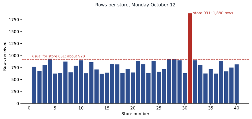
The row counts per store for Monday, October 12, show 39 stores between 600 and 950 rows, and store 031 with 1,880 rows. Its usual Monday count is about 920. What should Mateo do?
Show solution
- Compare with store 031's history: 1,880 is about twice its usual 920, which suggests duplication rather than a sudden boom.
- Count exact duplicate rows for store 031 on that day; if about 940 rows are exact copies, the till resent its whole day.
- Check with the store systems team whether the till reconnected after an outage.
- Make sure the staging deduplication rule removes the copies, and record the incident in the feed's log.
Answer: Treat a sudden doubling as likely duplication, confirm it by counting exact copies and checking with the source team, and let the deduplication rule handle it.
Summary and key terms
- Profiling inspects data to learn its shape and problems before cleaning and loading: row counts, empty rates, distinct counts, ranges, frequent values, patterns and distributions.
- External tables and scratch datasets with expiration let you query files before loading them permanently.
- APPROX_COUNT_DISTINCT and APPROX_QUANTILES profile large tables cheaply.
- Data profile scans in Dataplex Universal Catalog compute column statistics and can run on a schedule.
- On-demand queries are billed by bytes read, so choose fewer columns and use a dry run; LIMIT does not reduce bytes on a normal table.
- Findings must be interpreted with the data's owners before they become cleaning rules.
- Data profiling
- Systematically inspecting a dataset to learn its structure, content and quality.
- External table
- A BigQuery table definition that reads data where it is stored, such as files in Cloud Storage.
- Table expiration
- A setting that deletes a table automatically after a set time.
- Dry run
- A query check that reports the bytes a query would process without running it.
- APPROX_QUANTILES
- A BigQuery function that returns approximate values splitting data into equal parts.
- Data profile scan
- A Dataplex scan that computes statistics for each column of a table.
- Outlier
- A value far from the others, which may be an error or a real but rare event.
Practice problems
Work each problem on paper first, then reveal the answer to check.
Why profile data before writing cleaning rules?
Show answer
To learn which problems exist and how often, so the rules address real issues.
Does adding LIMIT 10 reduce the cost of a query on a normal BigQuery table?
Show answer
No; the bytes read depend on the columns selected, not on the rows returned.
What did the negative quantities in the till files turn out to be?
Show answer
Refunds recorded at the till.
Which tool can compute column statistics on a schedule and keep a history?
Show answer
A Dataplex data profile scan.
Lesson quiz · 5 questions
Score 60% or more to complete this lesson.
Create a free account to save your progress, take quizzes and earn a certificate.