
GCP-220 · Lesson 11 of 12 · 20 min
Choosing storage for prepared data
▶ Video coming soon A video version of this lesson is on the way.
Data that has been cleaned and checked has to live somewhere, and the right place depends on how it will be used. On Tuesday, November 10, Ravi gives Mateo a list of six things to store and asks him to choose a home for each: the raw till files, the curated sales tables, the 40 TB product photo library, the shop's live product catalog, a store-level stock table that the new mobile app will read thousands of times a minute, and seven years of tax records that must be kept but will almost never be read. No single service is right for all six.
Matching data to a storage service
The exam often describes a workload and asks for the storage service. The deciding questions are the shape of the data, how it is accessed, how much there is, and how fast reads and writes must be.
| Service | What it stores | Access pattern | Birchline fit |
|---|---|---|---|
| Cloud Storage | Objects (files) of any kind | Whole files read and written; no queries inside them | Raw landing files, product photos, archives, exports |
| BigQuery | Tables for analytics | SQL over large volumes, mostly reads and appends | Raw, staging and curated datasets; reports |
| Cloud SQL | Relational tables (MySQL, PostgreSQL, SQL Server) | Transactions; many small reads and writes | The shop's order and catalog database after migration |
| AlloyDB | PostgreSQL-compatible relational tables | Demanding transactional and mixed analytical work | An option if the shop outgrows Cloud SQL |
| Spanner | Relational tables, globally consistent and horizontally scalable | Transactions at very large scale or across regions | More than Birchline needs today |
| Bigtable | Wide-column key-value data | Very high throughput reads and writes by key, low latency | Time series and high-volume lookups |
| Firestore | Documents (semi-structured) for applications | App reads and writes by document, real-time sync to devices | The mobile app's per-store stock view |
A common exam trap is choosing BigQuery for an application's day-to-day database. BigQuery is built for analysis: scanning millions of rows to compute a total. It is not built for an app that updates one order at a time thousands of times a minute. The reverse trap is running large analytical reports against Cloud SQL, which will be slow and will compete with the shop's customers for the database. Operational data lives in operational databases, and copies flow to BigQuery for analysis, which is exactly what Datastream does for the shop.
Cloud Storage: classes and lifecycle
Cloud Storage offers several storage classes. They have the same speed and durability; they differ in the monthly price of storing data, the price of reading it back, and the minimum storage duration, the period you pay for even if you delete the object sooner.
| Class | Minimum storage duration | Retrieval charge | Fits |
|---|---|---|---|
| Standard | None | None | Data read often, such as landing files being loaded |
| Nearline | 30 days | Yes | Data read about once a month or less |
| Coldline | 90 days | Yes, higher | Data read about once a quarter or less |
| Archive | 365 days | Yes, highest | Data kept for years and rarely or never read |
Data does not have to stay in one class. Object Lifecycle Management rules move objects to a colder class or delete them when conditions are met, such as an object's age. Autoclass goes further and moves each object between classes automatically based on how often it is actually read, which suits data whose access pattern nobody can predict. Birchline's landing bucket uses a lifecycle rule: till files stay in Standard for 30 days while they might be reloaded, move to Coldline, and are deleted after 400 days, a little over the 13 months Finance wants to be able to reprocess.
{
  "rule": [
    {"action": {"type": "SetStorageClass", "storageClass": "COLDLINE"},
     "condition": {"age": 30, "matchesStorageClass": ["STANDARD"]}},
    {"action": {"type": "Delete"},
     "condition": {"age": 400}}
  ]
}
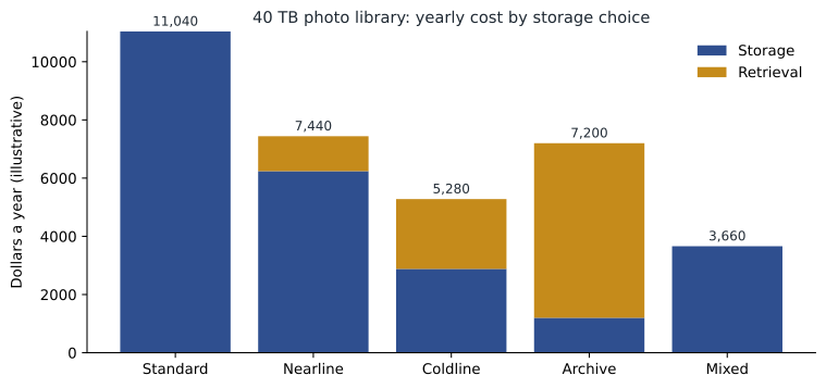
The photo library is a different case. Photos of current products are read constantly by the website and the merchandising team; photos of discontinued products are almost never read but must be kept for marketing archives. Nobody knows in advance which product will be discontinued, so Autoclass fits better than a fixed age rule. Mateo compares the yearly cost of a few options using illustrative prices, to see why the choice matters for 40 TB.
# Yearly storage cost for the 40 TB photo library under different choices (illustrative prices).
tb = 40
gb = tb * 1000
price_per_gb_month = {"Standard": 0.023, "Nearline": 0.013, "Coldline": 0.006, "Archive": 0.0025}
retrieval_per_gb   = {"Standard": 0.0,   "Nearline": 0.01,  "Coldline": 0.02,  "Archive": 0.05}
read_gb_per_year = 0.25 * gb * 12        # a quarter of the library read each month (current products)

for cls in price_per_gb_month:
    storage = gb * price_per_gb_month[cls] * 12
    reads = read_gb_per_year * retrieval_per_gb[cls]
    print(f"{cls:9s} storage {storage:8,.0f}  retrieval {reads:8,.0f}  total {storage + reads:8,.0f} dollars a year")

hot_share = 0.25   # roughly the current products, kept in Standard by Autoclass
mixed = gb * hot_share * price_per_gb_month["Standard"] * 12 + gb * (1 - hot_share) * price_per_gb_month["Archive"] * 12
print(f"Mixed (a quarter Standard, the rest Archive, few cold reads): about {mixed:,.0f} dollars a year")Standard storage 11,040 retrieval 0 total 11,040 dollars a year Nearline storage 6,240 retrieval 1,200 total 7,440 dollars a year Coldline storage 2,880 retrieval 2,400 total 5,280 dollars a year Archive storage 1,200 retrieval 6,000 total 7,200 dollars a year Mixed (a quarter Standard, the rest Archive, few cold reads): about 3,660 dollars a year
What this code does
It estimates a year of storing 40 TB in each storage class using illustrative monthly prices per gigabyte, and adds the cost of reading back a quarter of the library every month, since colder classes charge for each gigabyte read. It then estimates a mixed approach where the busy quarter of the photos stays in Standard and the rest sits in Archive. The comparison shows that a cold class is cheap only if the data is rarely read, and that keeping hot and cold data in different classes is cheapest of all.
The numbers make the point clearly. Standard for everything costs about 11,000 dollars a year. Archive looks cheapest for storage alone, at about 1,200 dollars, but reading a quarter of the library every month from Archive adds about 6,000 dollars of retrieval charges, which makes it dearer than Coldline at about 5,280 dollars in total. The mixed approach, which is roughly what Autoclass achieves on its own by keeping busy photos warm and letting the rest cool down, comes to about 3,660 dollars. The prices are illustrative and the real ones should be taken from the current price list for the chosen location, but the shape of the comparison holds: a cold class is cheap only for data that really is cold.
Location types
Every bucket and dataset has a location, and the exam guide asks you to choose among the types. A region is a single geographic place, such as us-east5 in Columbus. A dual-region is a specific pair of regions; data is replicated across both, so it survives the loss of one region and can be read in either. A multi-region is a large area, such as US, EU or ASIA, where Google chooses where to keep copies. A zone is a single data center area inside a region; Cloud Storage offers zonal buckets only for its Rapid storage, aimed at very high-performance AI and analytics work, and those buckets give up many features, including use with BigQuery.
| Location type | Availability | Performance | Typical use |
|---|---|---|---|
| Zonal (Rapid buckets) | One zone | Lowest latency, highest throughput next to compute in that zone | AI training data and checkpoints |
| Regional | Survives a zone failure | Best when compute is in the same region | Most data processed in one region, such as landing files |
| Dual-region | Survives a region failure | Good in both regions | Important data that must stay available and in a defined pair of places |
| Multi-region | Survives a region failure | Good for wide audiences | Content served to users across a continent |
For Birchline in the US, location is also a cost and resilience decision. The US multi-region spreads data widely, and Google also offers a predefined dual-region in North America, NAM4, pairing Iowa and South Carolina, as well as configurable dual-regions. The team uses regional Columbus buckets and datasets for analytics, to keep data next to BigQuery in us-east5, and a dual-region bucket for the photo library and for backups that must survive the loss of a region.
One rule ties location to the rest of the course: BigQuery loads and queries work best when the data and the dataset are in the same location, and some operations require it. A load from a bucket in one region into a dataset in another can fail or incur transfer charges. BigQuery data preparation, for example, requires its sources and destination to share a location, as lesson 4 noted. Choosing locations deliberately at the start saves painful moves later.
BigQuery storage
BigQuery storage has its own pricing rules that reward good table design. A table or partition that has not been modified for 90 consecutive days moves automatically to long-term storage, which costs about half as much, with no change in performance. Partitioning by date therefore saves money as well as query cost: last year's partitions become long-term storage while this month's stay active. A dataset can be billed on logical bytes (uncompressed) or physical bytes (compressed, including time travel data), and physical billing is often cheaper for data that compresses well.
BigQuery also keeps recent history. Time travel lets you query or restore a table as it was at any point in the last seven days by default, configurable down to two days, which is invaluable after a bad MERGE. After that, a further seven-day fail-safe period lets Google recover data in an emergency, though not on demand. And table expiration deletes tables or partitions automatically after a set time, which keeps scratch datasets from growing forever and enforces retention rules.
| Setting | Birchline choice | Reason |
|---|---|---|
| Dataset location | us-east5 | Same as the landing bucket and the team's other datasets |
| raw tables | Partitioned by date; partitions expire after 400 days | Matches the landing bucket's retention |
| scratch dataset | Default table expiration 7 days | Exploration tables clean themselves up |
| Time travel window | 7 days on curated, 2 days on scratch | Recovery for important tables; lower cost elsewhere |
| Storage billing model | Physical, after comparing estimates | Till and event data compress well |
Long-term retention
The seven years of tax records are a retention problem rather than an analytics one. Finance keeps seven years to cover federal and state requirements with room to spare. The records are exported as Parquet to an Archive-class bucket, and a retention policy on the bucket prevents anyone from deleting or overwriting objects before seven years have passed. Locking the policy makes it permanent, so it is done only after Finance and legal have agreed the period.
Mateo's answers
| Data | Home | Class or setting |
|---|---|---|
| Raw till files | Cloud Storage, regional | Standard for 30 days, then Coldline; deleted after 400 days |
| Curated sales tables | BigQuery, regional dataset | Partitioned by date; long-term pricing applies to old partitions |
| Product photo library | Cloud Storage, dual-region | Autoclass |
| Live product catalog | Cloud SQL (after migration from the data center) | Copied to BigQuery by Datastream |
| Store stock for the mobile app | Firestore | Documents per store and product, updated from the stock system |
| Seven years of tax records | Cloud Storage, Archive class | Retention policy of seven years, locked once agreed |
Common mistakes
MistakeUsing BigQuery as the database behind an app.
InsteadUse an operational database such as Cloud SQL or Firestore, and copy data to BigQuery for analysis.
MistakeChoosing Archive for data that is read every month.
InsteadCompare storage savings with retrieval charges; use Autoclass when the pattern is unknown.
MistakePutting a bucket and its BigQuery dataset in different locations.
InsteadKeep the data and the dataset in the same location.
MistakeDeleting objects in Nearline after a week and expecting to pay for a week.
InsteadRemember the minimum storage durations: 30, 90 and 365 days.
MistakeLocking a retention policy before the period is agreed.
InsteadA locked policy cannot be shortened or removed; agree the period first.
Worked problem
A home for the stock lookups
The new mobile app will show shoppers whether a product is in stock at their nearest store. Expect thousands of reads a minute at peak, updates whenever stock changes, and offline support on phones. The analytics team also wants daily stock history. Where should the data live?
Show solution
- The app reads and writes single records by key, at high rates, with real-time updates to phones; that is an operational, document-style workload.
- Firestore fits: documents per store and product, real-time listeners and offline support in its mobile libraries.
- BigQuery is wrong for the live lookups but right for history: a daily snapshot of stock levels can be exported to a partitioned BigQuery table.
- Keep both in the same country's regions, as required for Birchline's data.
Answer: Firestore for the live stock the app reads, with a daily copy to a partitioned BigQuery table for analysis.
Summary and key terms
- Choose storage by the shape of the data and how it is accessed: Cloud Storage for files, BigQuery for analytics, Cloud SQL, AlloyDB or Spanner for relational transactions, Bigtable for high-throughput key access and Firestore for app documents.
- Cloud Storage classes Standard, Nearline, Coldline and Archive have the same speed but different storage prices, retrieval charges and minimum durations of none, 30, 90 and 365 days.
- Lifecycle rules change class or delete by age; Autoclass moves objects by actual access.
- Locations can be zonal (Rapid buckets), regional, dual-region or multi-region; keep buckets and datasets in the same location.
- BigQuery moves untouched tables and partitions to cheaper long-term storage after 90 days, keeps time travel for up to seven days and supports table expiration.
- Retention policies protect records from deletion.
- Storage class
- A Cloud Storage pricing tier: Standard, Nearline, Coldline or Archive.
- Minimum storage duration
- The period you pay for even if an object is deleted sooner.
- Object Lifecycle Management
- Rules that change an object's class or delete it when conditions are met.
- Autoclass
- A Cloud Storage feature that moves objects between classes based on access.
- Dual-region
- A pair of regions where data is replicated so it survives the loss of one.
- Long-term storage
- Cheaper BigQuery storage for tables or partitions unmodified for 90 days.
- Time travel
- BigQuery's ability to query or restore a table as it was in the recent past.
- Retention policy
- A bucket setting that prevents deletion of objects before a set age.
Practice problems
Work each problem on paper first, then reveal the answer to check.
What are the minimum storage durations of Nearline, Coldline and Archive?
Show answer
30, 90 and 365 days.
When does BigQuery data move to long-term storage pricing?
Show answer
When a table or partition has not been modified for 90 consecutive days.
Which service suits a mobile app's per-store stock lookups?
Show answer
Firestore.
Why should a bucket and its BigQuery dataset share a location?
Show answer
Loads and queries work best, and some operations require it; crossing locations can fail or add charges.
Lesson quiz · 5 questions
Score 60% or more to complete this lesson.
Create a free account to save your progress, take quizzes and earn a certificate.