Magnetically coupled circuits and transformers

When two coils share magnetic flux, a changing current in one induces a voltage in the other, even though no conductor connects them. This magnetic coupling is how transformers change voltage levels throughout the power system, how isolated power supplies keep users safe from the mains, how current transformers let meters measure thousands of amperes, and how wireless chargers transfer energy. This lesson introduces mutual inductance and the dot convention, studies coupled coils in the frequency domain, develops the ideal transformer and impedance reflection, and builds the equivalent circuit of a practical transformer, with the tests used to find its parameters and the calculation of regulation and efficiency.

Mutual inductance

A coil with self-inductance \(L_1\) carrying current \(i_1\) produces flux, part of which links a second coil. The voltage induced in the second coil is proportional to the rate of change of \(i_1\):

where \(M\) is the mutual inductance, in henries, the same in both directions. It depends on the geometry of the coils and the magnetic material, and is limited by the self-inductances through the coupling coefficient \(k\):

Air-cored coils far apart have \(k\) near 0; coils wound together on an iron or ferrite core have \(k\) above 0.99. Wireless chargers operate with \(k\) of about 0.1 to 0.5, which is why their efficiency depends so much on alignment.

The dot convention

Whether the mutual voltage adds to or subtracts from the self-induced voltage depends on how the coils are wound, which a circuit diagram cannot show. The dot convention marks one terminal of each coil: if a current enters the dotted terminal of one coil, the mutual voltage it induces in the other coil is positive at that coil's dotted terminal. In equations, the mutual term has the same sign as the self term if both currents enter (or both leave) the dotted terminals, and the opposite sign otherwise.

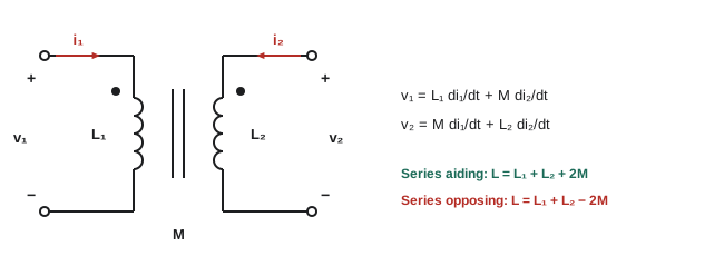
In the frequency domain, the coupled-coil equations become

A transformer with a load

Connecting a load impedance \(Z_L\) to the second coil and a source to the first gives the linear transformer. Writing the mesh equations, with \(I_1\) entering the dotted terminal of the primary and \(I_2\) leaving the dotted terminal of the secondary into the load:

Eliminating \(I_2\) shows that the source sees the primary impedance plus a reflected impedance:

The reflected impedance \(\omega^2M^2/(j\omega L_2 + Z_L)\) carries the effect of the secondary circuit into the primary. A resistive load reflects as a resistance (power delivered), and the reactance of the secondary reflects with its sign reversed.

The ideal transformer

An ideal transformer has perfect coupling (\(k = 1\)), infinite self-inductances, and no losses. It is described entirely by its turns ratio \(n = N_2/N_1\) (or \(a = N_1/N_2\), common in power engineering):

with currents defined so that power flows from primary to secondary. Voltage scales up by the turns ratio and current down by the same ratio, so complex power is conserved. The dots determine polarity: the voltages at the dotted terminals are in phase.

The most useful consequence is impedance transformation. A load \(Z_L\) on the secondary appears at the primary as

Referring quantities across the transformer

A circuit containing an ideal transformer is simplified by referring everything to one side: impedances are multiplied by \(a^2\) when moved from secondary to primary (divided when moved the other way), voltages by \(a\), and currents divided by \(a\). The transformer then disappears from the diagram, leaving an ordinary circuit. This is how power engineers analyze networks with many voltage levels, and the idea leads to the per-unit system (ELE-380).

The practical transformer

A real transformer departs from the ideal in four ways, each represented by an element in its equivalent circuit:

• Winding resistance \(R_1\), \(R_2\): copper losses that grow with the square of current.
• Leakage reactance \(X_1\), \(X_2\): flux that links only one winding, causing a voltage drop under load.
• Magnetizing reactance \(X_m\): the core needs a magnetizing current to establish flux, typically 1% to 5% of rated current.
• Core-loss resistance \(R_c\): hysteresis and eddy-current losses in the core, nearly constant at a given voltage and frequency.

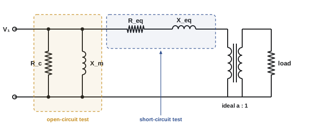
Because the magnetizing current is small, the shunt branch is often moved to the primary terminals, and the two windings' resistances and reactances are combined (referred to one side) into \(R_{eq}\) and \(X_{eq}\). This approximate circuit is accurate enough for most calculations.

Finding the parameters: open- and short-circuit tests

• Open-circuit test: rated voltage applied to one winding (usually the low-voltage side) with the other open. The current is just the magnetizing and core-loss current, and the measured power is the core loss. From V, I and P, \(R_c\) and \(X_m\) are found.
• Short-circuit test: the other winding is shorted and a reduced voltage (typically 2% to 10% of rated) is raised until rated current flows. Core loss is negligible at this low voltage, so the power measured is the copper loss at full load, and V, I and P give \(R_{eq}\) and \(X_{eq}\).

Regulation and efficiency

Voltage regulation is the rise in secondary voltage from full load to no load, as a percentage of the full-load voltage, with the primary voltage held constant. Efficiency is output power divided by input power. Both are calculated from the equivalent circuit:

import numpy as np

# Single-phase transformer 50 kVA, 2400/240 V, 60 Hz, referred to the high-voltage side
S_rated, V1, V2 = 50e3, 2400.0, 240.0
a = V1 / V2
Req, Xeq = 1.42, 1.82           # series impedance from the short-circuit test (HV side)
Rc, Xm = 50e3, 7.5e3            # core-loss and magnetizing branch from the open-circuit test

# Full load at 0.8 power factor lagging, rated secondary voltage
I2 = S_rated / V2                               # load current on the LV side
I2_ref = I2 / a * np.exp(-1j * np.arccos(0.8))  # referred to HV side, lagging
V2_ref = V2 * a                                 # 2400 V at angle 0
V1_needed = V2_ref + I2_ref * (Req + 1j * Xeq)
Ic = V1_needed / Rc
Im = V1_needed / (1j * Xm)
I1 = I2_ref + Ic + Im

reg = (abs(V1_needed) - V2_ref) / V2_ref * 100
P_out = S_rated * 0.8
P_cu = abs(I2_ref) ** 2 * Req
P_core = abs(V1_needed) ** 2 / Rc
eff = P_out / (P_out + P_cu + P_core) * 100
print(f"referred load current {abs(I2_ref):.2f} A; primary current {abs(I1):.2f} A")
print(f"primary voltage needed {abs(V1_needed):.1f} V at {np.degrees(np.angle(V1_needed)):.2f} deg")
print(f"voltage regulation {reg:.2f}%")
print(f"copper loss {P_cu:.0f} W, core loss {P_core:.0f} W, efficiency {eff:.2f}%")
# Efficiency is highest where copper loss equals core loss
x = np.sqrt(P_core / P_cu)
print(f"maximum efficiency at {100 * x:.0f}% of rated load")

referred load current 20.83 A; primary current 21.07 A
primary voltage needed 2446.4 V at 0.29 deg
voltage regulation 1.94%
copper loss 616 W, core loss 120 W, efficiency 98.19%
maximum efficiency at 44% of rated load

Efficiency peaks at the load where copper loss (which varies with the square of load) equals core loss (which is constant). Distribution transformers, which spend most of their lives lightly loaded, are designed with low core loss so that they are efficient at typical loads of 30% to 50%; efficiency regulations in Canada and the United States set minimum efficiencies at such reference loads.

Special transformers

• Autotransformers have a single winding with a tap, sharing part of the winding between input and output. For small voltage ratios they are smaller, cheaper and more efficient than two-winding transformers, but they provide no isolation.
• Instrument transformers scale large currents and voltages to safe levels for meters and relays: current transformers (CTs) typically give 5 A or 1 A at rated primary current, and voltage transformers (VTs) give 120 V. A CT secondary must never be opened while primary current flows, because the transformer then tries to drive its current into an open circuit, producing dangerous voltages.
• Isolation transformers with a 1:1 ratio separate a circuit from ground for safety or noise reduction.
• Three-phase transformers, made of three single-phase units or one three-limb core, connected in wye or delta (Lesson 7); their phase shifts and grounding are studied in ELE-380.