
ELE-203 · Lesson 11 of 12 · 28 min
Fourier series and non-sinusoidal waveforms
Phasor analysis assumes sinusoids, but many waveforms in electrical engineering are not sinusoidal: the square waves of inverters and digital clocks, the triangle waves of PWM generators, and the pulsed currents drawn by rectifiers in every computer, LED driver and variable-speed drive. Lesson 5 introduced harmonics and their effect on power. This lesson provides the underlying tool, the Fourier series, which represents any periodic waveform as a sum of sinusoids at multiples of its fundamental frequency. Combined with superposition (Lesson 4), it lets a circuit with a non-sinusoidal source be solved one harmonic at a time. The lesson then applies the method to power quality: total harmonic distortion, neutral currents from triplen harmonics, and true power factor.
The Fourier series
A periodic function \(f(t)\) with period \(T\) and fundamental angular frequency \(\omega_0 = 2\pi/T\) can be written as
with coefficients
The constant \(a_0\) is the average (DC) value; the \(n = 1\) terms are the fundamental; the others are harmonics. Each pair can be combined into one sinusoid of amplitude \(c_n = \sqrt{a_n^2 + b_n^2}\), and a plot of \(c_n\) against frequency is the waveform's amplitude spectrum.
Symmetry shortcuts
Symmetry eliminates terms before any integration:
- Even functions, \(f(-t) = f(t)\), have only cosine terms (\(b_n = 0\)).
- Odd functions, \(f(-t) = -f(t)\), have only sine terms (\(a_n = 0\)) and no DC.
- Half-wave symmetry, \(f(t + T/2) = -f(t)\), means only odd harmonics are present. Most waveforms in power systems have half-wave symmetry, which is why even harmonics are rare there and their presence (from half-wave rectification or transformer inrush) signals a problem.
Worked problem
Square wave
Find the Fourier series of a square wave equal to \(+A\) for the first half-period and \(-A\) for the second.
Show solution
- The wave is odd (taking t = 0 at a rising edge) and has half-wave symmetry: only odd sine terms.
- \(b_n = \frac{2}{T}\left[\int_0^{T/2} A\sin n\omega_0 t\,dt - \int_{T/2}^{T} A\sin n\omega_0 t\,dt\right] = \frac{4A}{n\pi}\) for odd \(n\).
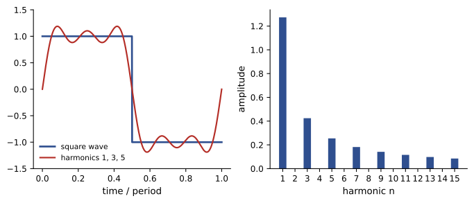
Answer: \(f(t) = \frac{4A}{\pi}\left(\sin\omega_0 t + \frac{1}{3}\sin 3\omega_0 t + \frac{1}{5}\sin 5\omega_0 t + \cdots\right)\). The harmonics fall as 1/n, slowly, because the square wave has jumps.
import numpy as np

# Fourier series of a square wave (amplitude 1, period T) computed numerically
T = 1 / 60
t = np.linspace(0, T, 20000, endpoint=False)
w0 = 2 * np.pi / T
sq = np.where(t < T / 2, 1.0, -1.0)

def coeffs(x, n):
    a = 2 * np.mean(x * np.cos(n * w0 * t))
    b = 2 * np.mean(x * np.sin(n * w0 * t))
    return a, b

print(" n   b_n numeric   4/(n pi)")
for n in range(1, 8):
    a, b = coeffs(sq, n)
    exact = 4 / (n * np.pi) if n % 2 else 0.0
    print(f"{n:2d}   {round(b, 4) + 0.0:10.4f}   {exact:9.4f}")

# Partial sums: rms error falls as harmonics are added
for N in (1, 3, 9, 49):
    approx = sum(4 / (n * np.pi) * np.sin(n * w0 * t) for n in range(1, N + 1, 2))
    err = np.sqrt(np.mean((sq - approx) ** 2))
print(f"harmonics up to {N:2d}: rms error {err:.3f}, peak {approx.max():.3f}")n b_n numeric 4/(n pi) 1 1.2732 1.2732 2 0.0000 0.0000 3 0.4244 0.4244 4 0.0000 0.0000 5 0.2546 0.2546 6 0.0000 0.0000 7 0.1819 0.1819 harmonics up to 1: rms error 0.435, peak 1.273 harmonics up to 3: rms error 0.315, peak 1.200 harmonics up to 9: rms error 0.201, peak 1.182 harmonics up to 49: rms error 0.090, peak 1.179
Two lessons follow. The smoother a waveform, the faster its harmonics decay: jumps give 1/n, kinks (like a triangle wave) give \(1/n^2\), and smooth waveforms decay faster still. And a finite sum overshoots near a jump by about 9% of the jump, however many terms are added (the Gibbs phenomenon), which is why filtered square waves show ringing at their edges.
Circuits with non-sinusoidal sources
Because a periodic source is a sum of sinusoids, the steady-state response of a linear circuit is found by superposition:
- Expand the source in a Fourier series and keep enough harmonics.
- For each harmonic \(n\), compute impedances at \(n\omega_0\): an inductor's reactance is \(n\) times its fundamental value; a capacitor's is \(1/n\) times.
- Find the response phasor at each harmonic, then add the time functions, or combine RMS values and powers as in Lesson 4.
Inductors therefore suppress high harmonics of current, while capacitors pass them. This is the principle of every filter used to clean up non-sinusoidal waveforms.
import numpy as np

# A 60 Hz square-wave inverter output (+/-100 V) drives an R-L load
Vdc, f, R, L = 100.0, 60.0, 5.0, 20e-3
w0 = 2 * np.pi * f
rows, Vh, Ih = [], [], []
for n in range(1, 40, 2):
    Vn = 4 * Vdc / (n * np.pi) / np.sqrt(2)      # rms of harmonic n
    Zn = abs(R + 1j * n * w0 * L)
    Vh.append(Vn); Ih.append(Vn / Zn)
    if n <= 9:
        rows.append((n, Vn, Zn, Vn / Zn))

print(" n   V_n rms   |Z_n|   I_n rms")
for n, V, Z, I in rows:
    print(f"{n:2d}  {V:8.2f}  {Z:6.2f}  {I:8.3f}")

Vh, Ih = np.array(Vh), np.array(Ih)
thd_v = np.sqrt(np.sum(Vh[1:] ** 2)) / Vh[0] * 100
thd_i = np.sqrt(np.sum(Ih[1:] ** 2)) / Ih[0] * 100
print(f"voltage THD {thd_v:.1f}%   current THD {thd_i:.1f}%")
print(f"rms current {np.sqrt(np.sum(Ih ** 2)):.2f} A; power {np.sum(Ih ** 2) * R:.0f} W, of which fundamental {Ih[0] ** 2 * R:.0f} W")n V_n rms |Z_n| I_n rms 1 90.03 9.05 9.952 3 30.01 23.17 1.295 5 18.01 38.03 0.473 7 12.86 53.02 0.243 9 10.00 68.04 0.147 voltage THD 47.0% current THD 14.2% rms current 10.05 A; power 505 W, of which fundamental 495 W
The voltage has 47% total harmonic distortion (48% with all harmonics included), but the current only 14%, because the impedance of the inductance rises with harmonic order. Almost all of the power, 495 W of 505 W, is delivered by the fundamental. This is how early inverters drove motors acceptably with square waves: the motor's inductance filtered the current.
Worked problem
Capacitor amplifying harmonics
A 20 µF capacitor is connected to a 240 V, 60 Hz supply whose voltage contains a 5th harmonic of 4% (9.6 V). Compare the fundamental and 5th harmonic currents.
Show solution
- Fundamental: \(X_C = 1/(2\pi \times 60 \times 20 \times 10^{-6}) = 132.6\) Ω; \(I_1 = 240/132.6 = 1.81\) A.
- 5th: \(X_C = 132.6/5 = 26.5\) Ω; \(I_5 = 9.6/26.5 = 0.362\) A.
- Current distortion from the 5th: \(0.362/1.81 = 20\%\), five times the voltage distortion.
Answer: A 4% voltage harmonic produces 20% current distortion in the capacitor. Power-factor-correction capacitors can be overloaded by harmonic currents, and can resonate with the system inductance near a harmonic; detuning reactors are added in series to prevent this.
Harmonic measures
The RMS value of a periodic waveform is the square root of the sum of the squares of the RMS values of its components:
Total harmonic distortion (THD) compares the harmonic content to the fundamental:
Voltage THD in public supplies is normally a few percent; IEEE 519 recommends limits of 5% at most points of connection to a utility below 69 kV, with separate limits for individual harmonics and for customers' current distortion. Current THD of single-phase electronic loads without power-factor correction is often 80% to over 100%.
Triplen harmonics and neutral currents
In a balanced three-phase system with identical non-linear loads on each phase, the \(n\)th harmonic of phase b is shifted by \(n \times 120°\) relative to phase a. For \(n\) = 3, 9, 15 (multiples of three, the triplen harmonics), the shift is a multiple of 360°: the triplen currents of the three phases are in phase and add in the neutral instead of canceling. Harmonics 5, 11, 17 form negative-sequence sets, and 7, 13, 19 positive-sequence sets (Lesson 8).
import numpy as np

# Current drawn by a single-phase rectifier load: harmonic magnitudes as % of fundamental
f = 60.0
harm = {1: 100.0, 3: 80.0, 5: 55.0, 7: 30.0, 9: 12.0, 11: 6.0}
I1 = 10.0                                  # fundamental rms, amperes
t = np.linspace(0, 1 / f, 4000, endpoint=False)

def phase_current(shift_deg):
    # each harmonic n is shifted by n times the phase shift
    return sum(I1 * pct / 100 * np.sqrt(2) * np.sin(n * (2 * np.pi * f * t - np.radians(shift_deg)))
               for n, pct in harm.items())

ia, ib, ic = phase_current(0), phase_current(120), phase_current(240)
rms = lambda x: np.sqrt(np.mean(x ** 2))
thd = np.sqrt(sum(p ** 2 for n, p in harm.items() if n > 1)) / 100
print(f"phase current rms {rms(ia):.2f} A, THD {100 * thd:.0f}%")
print(f"neutral current rms {rms(ia + ib + ic):.2f} A  ({rms(ia + ib + ic) / rms(ia):.2f} x phase)")
print(f"triplen check: 3 x sqrt(I3^2 + I9^2) = {3 * I1 * np.sqrt(0.8 ** 2 + 0.12 ** 2):.2f} A")

# True power factor = displacement factor x distortion factor
dpf = 0.98
distortion = 1 / np.sqrt(1 + thd ** 2)
print(f"distortion factor {distortion:.3f}; true power factor {dpf * distortion:.3f}")phase current rms 14.32 A, THD 102% neutral current rms 24.27 A (1.69 x phase) triplen check: 3 x sqrt(I3^2 + I9^2) = 24.27 A distortion factor 0.698; true power factor 0.684
This is why neutrals in buildings full of computers and LED lighting can carry more current than the phase conductors, overheating neutrals sized as if they would carry only unbalance, and why electrical codes count neutrals carrying harmonic currents as current-carrying conductors and allow or require oversized neutrals for such loads. Delta-wye transformers trap triplen currents in their delta windings, adding heat there; transformers serving such loads are often K-rated to tolerate it.
Power and power factor with harmonics
With a sinusoidal voltage, only the fundamental component of current delivers average power, but every harmonic adds to RMS current and therefore to losses and to the apparent power \(S = V_{rms}I_{rms}\). The true power factor is
the product of the displacement power factor (\(\cos\theta_1\), the angle between fundamental voltage and current) and the distortion factor. A rectifier load can have a displacement power factor of 0.98 yet a true power factor below 0.7, as the code example shows, and capacitors cannot correct it, because the problem is distortion, not phase shift. Active power-factor-correction circuits in modern power supplies shape the input current into a sinusoid, raising the true power factor above 0.95 (ELE-470).
Worked problem
Apparent power with harmonics
A 230 V supply feeds a load drawing a fundamental current of 8 A in phase with the voltage, plus harmonic currents totaling 6 A RMS. Find P, S and the power factor.
Show solution
- \(P = 230 \times 8 \times 1 = 1{,}840\) W.
- \(I_{rms} = \sqrt{8^2 + 6^2} = 10\) A; \(S = 230 \times 10 = 2{,}300\) VA.
- PF \(= 1{,}840/2{,}300 = 0.80\); THD \(= 6/8 = 75\%\); distortion factor \(1/\sqrt{1 + 0.5625} = 0.80\).
Answer: P = 1,840 W, S = 2,300 VA, PF = 0.80, entirely from distortion. The wiring and transformer must carry 10 A for 8 A of useful current.
Common mistakes
MistakeUsing phasors directly with a non-sinusoidal source.
InsteadExpand the source in a Fourier series and solve each harmonic separately.
MistakeUsing fundamental-frequency reactances for harmonics.
InsteadX_L scales with n and X_C with 1/n at harmonic n.
MistakeAssuming neutral current is small in balanced three-phase systems.
InsteadTriplen harmonics add in the neutral and can exceed phase current.
MistakeCorrecting a low power factor from distortion with capacitors.
InsteadDistortion needs filters or active PFC; capacitors may worsen harmonics.
MistakeMeasuring distorted currents with average-responding meters.
InsteadUse true-RMS instruments.
Summary and key terms
- Any periodic waveform is a DC term plus a fundamental and harmonics (the Fourier series).
- Symmetry removes terms; half-wave symmetry leaves only odd harmonics.
- Harmonics decay as 1/n for jumps and 1/n² for kinks; partial sums show Gibbs overshoot.
- Linear circuits with periodic sources are solved one harmonic at a time and added.
- RMS values add in quadrature; THD compares harmonic to fundamental content.
- Triplen harmonics add in neutrals; true PF = displacement factor × distortion factor.
- Fourier series
- A representation of a periodic function as a sum of sinusoids.
- Fundamental
- The component at the waveform's own frequency.
- Harmonic
- A component at an integer multiple of the fundamental frequency.
- Spectrum
- The amplitudes of a waveform's components plotted against frequency.
- Half-wave symmetry
- f(t + T/2) = −f(t), giving only odd harmonics.
- Gibbs phenomenon
- Persistent overshoot of Fourier partial sums at a jump.
- THD
- Total harmonic distortion: RMS of harmonics over the fundamental.
- Triplen harmonics
- Harmonics whose order is a multiple of three.
- Displacement power factor
- cos θ₁ between fundamental voltage and current.
- Distortion factor
- I₁/I_rms, the reduction in power factor due to harmonics.
Practice problems
Work each problem on paper first, then reveal the answer to check.
Third-harmonic amplitude of a ±10 V square wave?
Show answer
4.24 V peak.
Which harmonics does a waveform with half-wave symmetry contain?
Show answer
Odd harmonics only.
How fast do a triangle wave's harmonics decay?
Show answer
As 1/n².
Reactance of a 10 Ω (at 60 Hz) inductor at the 7th harmonic?
Show answer
70 Ω.
Reactance of a 50 Ω (at 60 Hz) capacitor at the 5th harmonic?
Show answer
10 Ω.
RMS of 10 A fundamental with 3 A 3rd and 4 A 5th?
Show answer
11.2 A.
THD for that current?
Show answer
50%.
Neutral current from three phases each carrying 6 A of 3rd harmonic?
Show answer
18 A.
True PF for displacement 0.95 and THD 60%?
Show answer
0.95/√1.36 = 0.81.
Why are even harmonics rare in power systems?
Show answer
Most waveforms have half-wave symmetry.
Lesson quiz · 5 questions
Score 60% or more to complete this lesson.
Create a free account to save your progress, take quizzes and earn a certificate.