
ELE-203 · Lesson 2 of 12 · 30 min
Second-order circuits
Lesson 1 introduced second-order circuits and classified their responses as overdamped, critically damped or underdamped. This lesson develops them fully. A circuit with two independent energy-storage elements, an inductor and a capacitor or two capacitors that cannot be combined, is described by a second-order differential equation, and its behavior, ringing, overshoot and settling, appears throughout electrical engineering: in power converter output filters, in the switching transients of contactors and circuit breakers, in signal integrity on printed circuit boards, and in every control loop. The method has four steps: write the differential equation, find the initial conditions, find the natural response, and add the forced response.
Writing the equations
For the series RLC circuit driven by a source \(v_s\), Kirchhoff's voltage law around the loop with \(i = C\,dv_C/dt\) gives an equation in the capacitor voltage:
with \(\alpha = R/(2L)\) and \(\omega_0 = 1/\sqrt{LC}\). For the parallel RLC circuit driven by a current source \(i_s\), Kirchhoff's current law with \(v = L\,di_L/dt\) gives the same form in the inductor current, with \(\alpha = 1/(2RC)\):
Every second-order circuit, however complicated, reduces to this standard form, which is why two numbers, \(\alpha\) and \(\omega_0\), describe its behavior. Engineers often use the dimensionless damping ratio \(\zeta = \alpha/\omega_0\) instead of \(\alpha\), and the quality factor \(Q = 1/(2\zeta)\):
| Case | Damping ratio | Roots of the characteristic equation | Natural response |
|---|---|---|---|
| Overdamped | \(\zeta > 1\) | Two real, negative: \(s_{1,2} = -\alpha \pm \sqrt{\alpha^2 - \omega_0^2}\) | \(A_1 e^{s_1 t} + A_2 e^{s_2 t}\) |
| Critically damped | \(\zeta = 1\) | Repeated: \(s = -\alpha\) | \((A_1 + A_2 t)e^{-\alpha t}\) |
| Underdamped | \(\zeta < 1\) | Complex: \(s = -\alpha \pm j\omega_d\) | \(e^{-\alpha t}(B_1\cos\omega_d t + B_2\sin\omega_d t)\) |
Initial conditions
The two constants in the natural response are found from two initial conditions: the value of the variable and of its first derivative just after switching, at \(t = 0^+\). They come from the continuity rules of Lesson 1:
- Capacitor voltage and inductor current cannot change instantly, so \(v_C(0^+) = v_C(0^-)\) and \(i_L(0^+) = i_L(0^-)\), found from the circuit before switching (in DC steady state, a capacitor is an open circuit and an inductor a short circuit).
- The derivatives come from the element laws: \(dv_C/dt(0^+) = i_C(0^+)/C\) and \(di_L/dt(0^+) = v_L(0^+)/L\), where \(i_C(0^+)\) and \(v_L(0^+)\) are found by analyzing the circuit at \(t = 0^+\), with each capacitor replaced by a voltage source equal to its initial voltage and each inductor by a current source equal to its initial current.
Worked problem
Finding initial conditions
In a series RLC circuit (R = 4 Ω, L = 1 mH, C = 10 µF), the capacitor is charged to 6 V and the inductor current is 0 when a switch connects a 10 V source at t = 0. Find \(v_C(0^+)\) and \(dv_C/dt(0^+)\).
Show solution
- Continuity: \(v_C(0^+) = 6\) V and \(i(0^+) = 0\).
- The current through the capacitor is the series current: \(i_C(0^+) = 0\).
- So \(dv_C/dt(0^+) = 0/C = 0\) V/s.
- And the inductor voltage at \(0^+\) is \(10 - 4 \times 0 - 6 = 4\) V, so \(di/dt(0^+) = 4/0.001 = 4{,}000\) A/s.
Answer: \(v_C(0^+) = 6\) V, \(dv_C/dt(0^+) = 0\). The current starts at zero but rises at 4,000 A/s, which is what drives the capacitor voltage away from 6 V.
The step response
When a constant source is switched on, the complete response is the sum of a forced (steady-state) response, here the final value \(v_C(\infty)\), and the natural response:
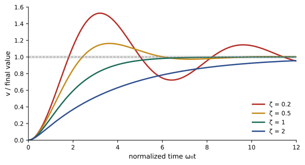
For the series RLC circuit driven by a step \(V_s\), \(v_C(\infty) = V_s\), because in steady state the capacitor blocks DC and no current flows. With zero initial conditions, the underdamped step response is
Measures of the step response
For an underdamped response, a few numbers summarize performance, and they are used everywhere from power supplies to control systems:
- Percent overshoot: \(\mathrm{PO} = 100\,e^{-\pi\zeta/\sqrt{1-\zeta^2}}\) %, which depends only on \(\zeta\).
- Peak time: \(t_p = \pi/\omega_d\), when the first maximum occurs.
- Settling time: the time to stay within a band (often 2%) of the final value, approximately \(t_s \approx 4/\alpha\).
- Rise time: the time to go from 10% to 90% of the final value.
import numpy as np

# Series RLC driven by a 10 V step; output is the capacitor voltage
R, L, C, Vs = 4.0, 1e-3, 10e-6, 10.0
alpha = R / (2 * L)
w0 = 1 / np.sqrt(L * C)
zeta = alpha / w0
wd = w0 * np.sqrt(1 - zeta ** 2)
print(f"alpha {alpha:.0f} 1/s, w0 {w0:.0f} rad/s, zeta {zeta:.3f}, wd {wd:.0f} rad/s")

# Analytic underdamped step response with v(0) = 0 and i(0) = 0
t = np.linspace(0, 3e-3, 30001)
v = Vs * (1 - np.exp(-alpha * t) * (np.cos(wd * t) + alpha / wd * np.sin(wd * t)))

# Numerical check: integrate the state equations with small time steps
dt = t[1] - t[0]
vc, i = 0.0, 0.0
vn = np.empty_like(t)
for k in range(len(t)):
    vn[k] = vc
    di = (Vs - R * i - vc) / L
    i += di * dt
    vc += i / C * dt
print(f"largest difference analytic vs numerical: {np.max(np.abs(v - vn)):.3f} V")

peak = v.max()
tp = t[v.argmax()]
outside = np.where(np.abs(v - Vs) > 0.02 * Vs)[0]
ts = t[outside[-1]]
print(f"peak {peak:.2f} V at {tp * 1e3:.3f} ms, overshoot {100 * (peak / Vs - 1):.1f}%")
print(f"formula overshoot {100 * np.exp(-np.pi * zeta / np.sqrt(1 - zeta ** 2)):.1f}%, peak time {np.pi / wd * 1e3:.3f} ms")
print(f"2% settling time {ts * 1e3:.2f} ms (estimate 4/alpha = {4 / alpha * 1e3:.2f} ms)")alpha 2000 1/s, w0 10000 rad/s, zeta 0.200, wd 9798 rad/s largest difference analytic vs numerical: 0.005 V peak 15.27 V at 0.321 ms, overshoot 52.7% formula overshoot 52.7%, peak time 0.321 ms 2% settling time 1.96 ms (estimate 4/alpha = 2.00 ms)
The numerical integration uses a simple update of the circuit's two state variables, the inductor current and capacitor voltage, each time step. It agrees with the formula to a few millivolts, and the same approach works for circuits with no closed-form solution, which is how circuit simulators such as SPICE work (Lesson 12).
Worked problem
Designing for overshoot
An LC output filter of a converter has L = 22 µH and C = 100 µF. The load and wiring add an effective series resistance R. What R gives 5% overshoot to a step in the input?
Show solution
- For 5% overshoot: \(\ln(0.05) = -\pi\zeta/\sqrt{1-\zeta^2}\), so \(\zeta = 0.69\).
- \(\omega_0 = 1/\sqrt{22 \times 10^{-6} \times 100 \times 10^{-6}} = 21{,}320\) rad/s (3.39 kHz).
- \(\alpha = \zeta\omega_0 = 14{,}710\) s⁻¹; \(R = 2L\alpha = 2 \times 22 \times 10^{-6} \times 14{,}710 = 0.65\) Ω.
Answer: About 0.65 Ω. Real filters have much less resistance, so they ring strongly unless damping is added, for example a resistor in series with an extra capacitor across the output, which damps the resonance without wasting DC power.
Overdamped and critically damped responses
For \(\zeta \geq 1\) the response does not oscillate. An overdamped response has two time constants, \(1/|s_1|\) and \(1/|s_2|\); the slower one dominates after the first moments. Increasing damping beyond critical makes the response slower, not faster: a heavily overdamped circuit behaves almost like a first-order circuit with a long time constant. Critical damping (\(\zeta = 1\)) gives the fastest response with no overshoot, but in practice a slightly underdamped design (\(\zeta\) about 0.7) is often preferred, because it is faster still and its overshoot of about 4.6% is acceptable.
Worked problem
An overdamped parallel RLC circuit
A parallel RLC circuit has R = 50 Ω, L = 0.2 H and C = 10 µF. Find \(\alpha\), \(\omega_0\), and the roots of the characteristic equation. Which time constant dominates?
Show solution
- \(\alpha = 1/(2RC) = 1/(2 \times 50 \times 10^{-5}) = 1{,}000\) s⁻¹.
- \(\omega_0 = 1/\sqrt{0.2 \times 10^{-5}} = 707\) rad/s; \(\zeta = 1.41\), overdamped.
- \(s_{1,2} = -1000 \pm \sqrt{1000^2 - 707^2} = -1000 \pm 707\): \(s_1 = -293\), \(s_2 = -1707\) s⁻¹.
- Time constants: 3.41 ms and 0.59 ms.
Answer: Roots −293 and −1,707 s⁻¹. The slower term, with time constant 3.41 ms, dominates after about a millisecond, and the response takes about 5 × 3.41 = 17 ms to settle.
Other second-order circuits
The same analysis applies to circuits that are not simple series or parallel RLC combinations:
- Circuits with two capacitors (or two inductors) separated by resistance, such as two-stage RC filters. Without an inductor, the roots are always real and the response cannot oscillate, unless an active element is present.
- Op-amp circuits with two capacitors, such as the Sallen-Key filter (Lesson 9), which can realize any damping ratio, including underdamped responses, without inductors.
- Mechanical, hydraulic and thermal systems with the same equations, such as a mass, spring and damper, which is why electrical analogies are used to model them.
For a general circuit, write state equations: one first-order equation for each capacitor voltage and inductor current, from KCL and KVL. Eliminating one variable gives the second-order equation, or the state equations can be solved directly, as in the code above.
Worked problem
Two-capacitor circuit
Two RC sections are cascaded: \(R_1 = R_2 = 10\) kΩ and \(C_1 = C_2 = 10\) nF. Its characteristic equation is \(s^2 + s\left(\frac{1}{R_1C_1} + \frac{1}{R_2C_2} + \frac{1}{R_2C_1}\right) + \frac{1}{R_1R_2C_1C_2} = 0\). Find the roots and the damping ratio.
Show solution
- \(1/(RC) = 10^{4}\) s⁻¹, so the middle coefficient is \(3 \times 10^{4}\) and the last \(10^{8}\).
- \(\omega_0 = 10^{4}\) rad/s; \(2\alpha = 3 \times 10^{4}\), \(\alpha = 1.5 \times 10^{4}\), \(\zeta = 1.5\).
- Roots: \(s = -1.5 \times 10^{4} \pm \sqrt{2.25 - 1} \times 10^{4} = -3{,}820\) and \(-26{,}180\) s⁻¹.
Answer: Two real roots; \(\zeta = 1.5\). Passive RC networks are always overdamped, which is why active filters (Lesson 9) or inductors are needed for sharper responses.
Where second-order behavior matters
- Switching transients: when a breaker closes onto a capacitor bank, or a contactor opens an inductive load, the circuit's inductance and capacitance ring at high frequency, producing overvoltages that can reach twice the supply peak. Snubbers (RC networks across switches) and pre-insertion resistors add damping.
- Power converter filters: the LC filters at the outputs and inputs of switch-mode supplies resonate, and their peaking must be damped to keep the converter's control loop stable.
- Signal integrity: a fast digital edge driving a trace or cable with stray inductance and capacitance rings, causing false switching; series termination resistors provide damping.
- Instrumentation: measurement systems such as accelerometers and pressure sensors are second-order, and their damping determines how faithfully they follow fast changes.
Common mistakes
MistakeUsing only the initial value of the variable.
InsteadA second-order response needs two initial conditions: the value and its derivative at 0⁺.
MistakeAssuming more damping always means faster settling.
InsteadBeyond critical damping the response slows; ζ ≈ 0.7 is often fastest with small overshoot.
MistakeUsing α = R/(2L) for a parallel RLC circuit.
InsteadFor parallel RLC, α = 1/(2RC).
MistakeExpecting an RC-only network to ring.
InsteadPassive RC networks have real roots; oscillation needs inductance or an active element.
MistakeConfusing ω₀ with the frequency of ringing.
InsteadThe ringing frequency is ω_d = √(ω₀² − α²), slightly below ω₀.
Summary and key terms
- Every second-order circuit reduces to x″ + 2αx′ + ω₀²x = forcing.
- Series RLC: α = R/2L; parallel RLC: α = 1/2RC; ω₀ = 1/√LC; ζ = α/ω₀; Q = 1/2ζ.
- Initial value and derivative at 0⁺ come from continuity and the element laws.
- Step response = final value + natural response.
- Overshoot depends only on ζ; peak time π/ω_d; settling time about 4/α.
- Second-order ringing appears in switching transients, converter filters and signal integrity.
- Second-order circuit
- A circuit described by a second-order differential equation.
- Neper frequency
- The damping coefficient α, in s⁻¹.
- Undamped natural frequency
- ω₀ = 1/√LC.
- Damped frequency
- ω_d, the frequency of ringing in an underdamped response.
- Damping ratio
- ζ = α/ω₀.
- Quality factor
- Q = 1/(2ζ), a measure of how lightly damped a circuit is.
- Percent overshoot
- How far the response exceeds its final value, as a percentage.
- Settling time
- The time for the response to stay within a band of its final value.
- State variables
- Capacitor voltages and inductor currents that describe a circuit's energy.
- Snubber
- A network that damps switching transients.
Practice problems
Work each problem on paper first, then reveal the answer to check.
Series RLC with R = 20 Ω, L = 5 mH, C = 2 µF: α, ω₀, ζ?
Show answer
2,000 s⁻¹; 10,000 rad/s; 0.2.
Parallel RLC with R = 1 kΩ, C = 1 µF: α?
Show answer
500 s⁻¹.
Q for ζ = 0.1?
Show answer
5.
Percent overshoot for ζ = 0.5?
Show answer
16.3%.
Peak time for ω_d = 5,000 rad/s?
Show answer
0.628 ms.
Settling time estimate for α = 250 s⁻¹?
Show answer
16 ms.
What resistance critically damps L = 1 mH, C = 1 µF in series?
Show answer
2√(L/C) = 63.2 Ω.
Roots for α = 500, ω₀ = 300?
Show answer
−100 and −900 s⁻¹.
Why does a passive RC ladder never ring?
Show answer
Its characteristic roots are always real.
di/dt at 0⁺ if v_L(0⁺) = 12 V and L = 3 mH?
Show answer
4,000 A/s.
Lesson quiz · 5 questions
Score 60% or more to complete this lesson.
Create a free account to save your progress, take quizzes and earn a certificate.