
ELE-203 · Lesson 10 of 12 · 26 min
Circuit analysis with the Laplace transform
The methods of the earlier lessons each handle one kind of problem: time-domain differential equations for transients (Lessons 1 and 2), phasors for sinusoidal steady state (Lessons 3 to 8), and frequency response for filters (Lesson 9). The Laplace transform unifies them. It turns differential equations into algebraic equations, includes initial conditions automatically, gives the complete response (transient and steady state) to any input, and leads to the transfer function, whose poles and zeros describe a circuit's behavior in both time and frequency. This lesson introduces the transform and its properties, circuit elements in the s-domain, partial-fraction inversion, transfer functions, and stability. ELE-250 develops the transform further for signals and systems.
The Laplace transform
The (one-sided) Laplace transform of a function \(f(t)\) defined for \(t \ge 0\) is
where \(s = \sigma + j\omega\) is the complex frequency. Starting the integral at \(0^-\) includes any impulse at \(t = 0\) and makes the initial conditions those just before switching, which are known. In practice, transforms are taken from a table:
| f(t), t ≥ 0 | F(s) |
|---|---|
| \(\delta(t)\) (unit impulse) | \(1\) |
| \(u(t)\) (unit step) | \(1/s\) |
| \(t\) | \(1/s^2\) |
| \(e^{-at}\) | \(1/(s + a)\) |
| \(t e^{-at}\) | \(1/(s + a)^2\) |
| \(\sin\omega t\) | \(\omega/(s^2 + \omega^2)\) |
| \(\cos\omega t\) | \(s/(s^2 + \omega^2)\) |
| \(e^{-at}\cos\omega t\) | \((s + a)/((s + a)^2 + \omega^2)\) |
| \(e^{-at}\sin\omega t\) | \(\omega/((s + a)^2 + \omega^2)\) |
The properties that make the transform useful for circuits are:
- Linearity: \(\mathcal{L}\{af + bg\} = aF + bG\).
- Differentiation: \(\mathcal{L}\{df/dt\} = sF(s) - f(0^-)\). Differentiation becomes multiplication by \(s\), with the initial value appearing automatically.
- Integration: \(\mathcal{L}\{\int_0^t f\,d\tau\} = F(s)/s\).
- Time shift: \(\mathcal{L}\{f(t - T)u(t - T)\} = e^{-sT}F(s)\), for delayed inputs such as pulses.
- Initial and final values: \(f(0^+) = \lim_{s\to\infty} sF(s)\) and, if the final value exists, \(f(\infty) = \lim_{s\to 0} sF(s)\).
Circuit elements in the s-domain
Transforming each element's equation gives an s-domain model, in which initial conditions appear as sources:
- Resistor: \(V = RI\).
- Inductor: \(V = sLI - L\,i(0^-)\): an impedance \(sL\) in series with a voltage source \(L\,i(0^-)\) (or in parallel with a current source \(i(0^-)/s\)).
- Capacitor: \(V = I/(sC) + v(0^-)/s\): an impedance \(1/(sC)\) in series with a voltage source \(v(0^-)/s\) (or in parallel with a current source \(C\,v(0^-)\)).
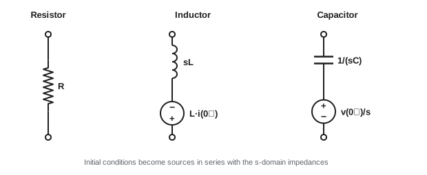
With these models, a circuit is analyzed exactly as in the phasor domain, with impedances \(R\), \(sL\) and \(1/(sC)\), using nodal, mesh, Thévenin or any other method. Setting \(s = j\omega\) recovers the phasor impedances, which shows that phasor analysis is a special case.
Inverting by partial fractions
For circuits, the transformed response is a ratio of polynomials in \(s\). It is inverted by expanding into partial fractions, each of which appears in the table:
The \(p_k\) are the poles (roots of the denominator) and the \(r_k\) the residues, found by \(r_k = [(s - p_k)F(s)]_{s = p_k}\). Complex poles come in conjugate pairs with conjugate residues, and each pair combines into a damped sinusoid. Repeated poles give terms in \(t e^{pt}\).
Worked problem
An RC circuit by Laplace
A 1 µF capacitor charged to 4 V is connected at t = 0 through a 2 kΩ resistor to a 10 V source. Find \(v_C(t)\).
Show solution
- Loop: \(10/s = 2000\,I + I/(10^{-6}s) + 4/s\), so \(I(s) = (6/s)/(2000 + 10^{6}/s) = 0.003/(s + 500)\).
- \(V_C(s) = I/(sC) + 4/s = 3000/(s(s + 500)) + 4/s\).
- Partial fractions: \(3000/(s(s + 500)) = 6/s - 6/(s + 500)\).
- \(V_C(s) = 10/s - 6/(s + 500)\), so \(v_C(t) = 10 - 6e^{-500t}\) V.
Answer: \(v_C(t) = 10 - 6e^{-500t}\) V, from 4 V toward 10 V with τ = 2 ms, the same result the first-order method of Lesson 1 gives directly, but obtained mechanically with the initial condition included.
The same mechanics apply to the second-order example of Lesson 2:
import numpy as np
from scipy import signal

# Series RLC (R = 4, L = 1 mH, C = 10 uF) with v_C(0) = 6 V, i(0) = 0 and a 10 V step at t = 0.
# s-domain: (10/s - 6/s) = I(s) (R + sL + 1/(sC))  ->  V_C(s) = 6/s + I(s)/(sC)
R, L, C = 4.0, 1e-3, 10e-6
# V_C(s) = [10 w0^2 + 6 s^2 + 6 (R/L) s] / [s (s^2 + (R/L) s + w0^2)]
w02 = 1 / (L * C)
num = [6.0, 6.0 * R / L, 10.0 * w02]
den = np.polymul([1.0, 0.0], [1.0, R / L, w02])
r, p, k = signal.residue(num, den)
for ri, pi in zip(r, p):
    print(f"pole {pi.real:9.1f} {pi.imag:+10.1f}j   residue {ri.real:7.3f} {ri.imag:+7.3f}j")

# Initial and final value theorems
print("initial value v_C(0+) = lim s V(s) as s -> inf =", num[0] / den[0])
print("final value  v_C(inf) = lim s V(s) as s -> 0  =", num[-1] / w02)

# Time response from the residues, checked against scipy
t = np.linspace(0, 2e-3, 2001)
v = np.real(sum(ri * np.exp(pi * t) for ri, pi in zip(r, p)))
_, v_check = signal.impulse((num, den), T=t)
print(f"v_C at 0.1, 0.3, 1.0 ms: {np.interp([1e-4, 3e-4, 1e-3], t, v).round(2)} V")
print(f"max difference from scipy.signal.impulse: {np.max(np.abs(v - v_check)):.1e} V")pole 0.0 +0.0j residue 10.000 +0.000j pole -2000.0 +9798.0j residue -2.000 +0.408j pole -2000.0 -9798.0j residue -2.000 -0.408j initial value v_C(0+) = lim s V(s) as s -> inf = 6.0 final value v_C(inf) = lim s V(s) as s -> 0 = 10.0 v_C at 0.1, 0.3, 1.0 ms: [ 7.62 12.06 10.54] V max difference from scipy.signal.impulse: 8.3e-14 V
The pole at \(s = 0\) with residue 10 is the final value (the forced response); the complex pair at \(-2000 \pm j9798\) gives the damped ringing (the natural response). The initial-value theorem confirms that \(v_C(0^+) = 6\) V, the capacitor's initial charge, and the final-value theorem that it settles at 10 V.
Transfer functions
With all initial conditions zero, the ratio of the transformed output to the transformed input is the transfer function:
The roots of the numerator are the zeros and those of the denominator the poles. The transfer function contains everything about the circuit's input-output behavior:
- The impulse response is \(h(t) = \mathcal{L}^{-1}\{H(s)\}\); the response to any input is \(Y(s) = H(s)X(s)\), or the convolution \(y = h * x\) in time.
- The frequency response is \(H(j\omega)\), evaluated on the imaginary axis (Lesson 9).
- The poles determine the natural response: each pole contributes a term \(e^{p t}\).
Poles and stability
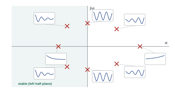
A circuit is stable if its natural response decays, which requires every pole to have a negative real part, in the left half of the s-plane. Poles on the imaginary axis give sustained oscillation (marginal stability), and poles in the right half-plane give responses that grow until something limits them.
Passive RLC circuits are always stable, because resistance only removes energy. Circuits with active elements, such as op-amps, transistors and dependent sources, can supply energy and become unstable. This is how oscillators are designed (deliberately placing poles on the imaginary axis) and how amplifiers and control loops fail (accidentally placing poles in the right half-plane).
import numpy as np
from scipy import signal

# H(s) = V_C / V_in for a series RLC: w0^2 / (s^2 + (R/L) s + w0^2), L = 1 mH, C = 10 uF
L, C = 1e-3, 10e-6
w0 = 1 / np.sqrt(L * C)
for R in (40.0, 20.0, 4.0, 0.0, -2.0):
    poles = np.roots([1.0, R / L, w0 ** 2])
    if np.all(poles.real < 0):
        kind = "stable"
    elif np.all(poles.real <= 0):
        kind = "marginal: sustained oscillation"
    else:
        kind = "unstable: growing oscillation"
    zeta = R / (2 * L) / w0
    p = ", ".join(f"{q.real + 0.0:8.0f}{q.imag:+8.0f}j" for q in poles)
    print(f"R = {R:5.1f} ohm  zeta = {zeta:5.2f}  poles {p}  {kind}")

# Frequency response from the transfer function for R = 4 ohm
sys = signal.TransferFunction([w0 ** 2], [1.0, 4.0 / L, w0 ** 2])
w, mag, phase = signal.bode(sys, w=[1e3, 1e4, 1e5])
for wi, m, ph in zip(w, mag, phase):
print(f"w = {wi:8.0f} rad/s |H| = {m:6.1f} dB phase = {ph:7.1f} deg")R = 40.0 ohm zeta = 2.00 poles -37321 +0j, -2679 +0j stable R = 20.0 ohm zeta = 1.00 poles -10000 +0j, -10000 +0j stable R = 4.0 ohm zeta = 0.20 poles -2000 +9798j, -2000 -9798j stable R = 0.0 ohm zeta = 0.00 poles 0 +10000j, 0 -10000j marginal: sustained oscillation R = -2.0 ohm zeta = -0.10 poles 1000 +9950j, 1000 -9950j unstable: growing oscillation w = 1000 rad/s |H| = 0.1 dB phase = -2.3 deg w = 10000 rad/s |H| = 8.0 dB phase = -90.0 deg w = 100000 rad/s |H| = -39.9 dB phase = -177.7 deg
The sequence shows the poles moving from two real values (overdamped), to a repeated pole (critically damped), to a complex pair (underdamped), onto the imaginary axis (R = 0, a lossless LC oscillator) and into the right half-plane when the resistance becomes negative, as it effectively does in the active circuit of an oscillator.
Worked problem
Transfer function of an RC low-pass filter
Find \(H(s) = V_o/V_i\) for a series R feeding a shunt C, with R = 1 kΩ and C = 1 µF. Find its pole, its step response, and its frequency response at the pole frequency.
Show solution
- Voltage divider: \(H(s) = (1/sC)/(R + 1/sC) = 1/(1 + sRC) = 1000/(s + 1000)\).
- Pole at \(s = -1000\) s⁻¹; no finite zeros.
- Step: \(Y = 1000/(s(s + 1000)) = 1/s - 1/(s + 1000)\), so \(y(t) = 1 - e^{-1000t}\).
- At \(\omega = 1000\): \(H(j1000) = 1/(1 + j) = 0.707\angle{-45°}\).
Answer: One pole at −1,000 s⁻¹ fixes both the time constant (1 ms) and the corner frequency (1,000 rad/s, where the gain is −3 dB): the time and frequency descriptions are two views of the same pole.
Choosing a method
With several tools available, the choice depends on the question:
- DC or sinusoidal steady state only: DC analysis or phasors.
- First-order transients with step inputs: the inspection method of Lesson 1 is fastest.
- Second-order or higher transients, arbitrary inputs, or initial conditions with several elements: Laplace.
- Frequency response and filter design: transfer functions and Bode plots.
- Non-linear circuits or large networks: numerical simulation (Lesson 12).
Common mistakes
MistakeForgetting the initial-condition sources in s-domain models.
InsteadInclude L·i(0⁻) and v(0⁻)/s sources for energized elements.
MistakeApplying the final-value theorem when poles lie on the imaginary axis or in the right half-plane.
InsteadUse it only when all poles of sF(s) are in the left half-plane.
MistakeInverting complex-pole terms separately as real exponentials.
InsteadCombine conjugate pairs into damped sinusoids.
MistakeIncluding initial conditions in a transfer function.
InsteadTransfer functions assume zero initial conditions.
MistakeAssuming active circuits are stable like passive ones.
InsteadCheck that all poles have negative real parts.
Summary and key terms
- The Laplace transform turns differential equations into algebra and includes initial conditions.
- In the s-domain, L becomes sL with a source L·i(0⁻), and C becomes 1/sC with a source v(0⁻)/s.
- Responses are inverted by partial fractions: each pole p contributes r·e^(pt).
- Initial- and final-value theorems check results quickly.
- Transfer functions H(s) give impulse, step and frequency responses; poles set the natural response.
- Stability requires all poles in the left half-plane.
- Laplace transform
- An integral transform from functions of time to functions of complex frequency s.
- Complex frequency
- s = σ + jω.
- s-domain
- The representation of a circuit after Laplace transformation.
- Partial fractions
- A sum of simple terms used to invert a rational transform.
- Residue
- The coefficient of a partial-fraction term.
- Transfer function
- The ratio of output to input transforms with zero initial conditions.
- Pole
- A root of a transfer function's denominator.
- Zero
- A root of a transfer function's numerator.
- Impulse response
- The output when the input is a unit impulse; the inverse transform of H(s).
- Stability
- The property that natural responses decay.
Practice problems
Work each problem on paper first, then reveal the answer to check.
Transform of 5e^(−3t)?
Show answer
5/(s + 3).
Inverse of 2/(s(s + 2))?
Show answer
1 − e^(−2t).
Inverse of (s + 2)/((s + 2)² + 9)?
Show answer
e^(−2t)cos 3t.
s-domain model of a 10 mH inductor carrying 2 A at 0⁻?
Show answer
Impedance 0.01s in series with a 0.02 V source.
s-domain source for a capacitor at 5 V?
Show answer
5/s in series with 1/(sC).
Final value of 20/(s(s + 4))?
Show answer
5.
Initial value f(0⁺) if F(s) = (3s + 1)/(s(s + 2))?
Show answer
3.
Poles of H = 1/(s² + 6s + 25)?
Show answer
−3 ± j4.
Is H = 1/(s² − s + 4) stable?
Show answer
No; its poles have positive real parts.
Time constant and corner frequency for a pole at −250 s⁻¹?
Show answer
4 ms; 250 rad/s.
Lesson quiz · 5 questions
Score 60% or more to complete this lesson.
Create a free account to save your progress, take quizzes and earn a certificate.