Sinusoidal steady-state analysis

Lesson 3 showed that, in sinusoidal steady state, phasors turn differential equations into algebra: each element becomes an impedance, and Ohm's and Kirchhoff's laws hold for complex voltages and currents. That means every DC analysis method from ELE-202 carries over to AC circuits unchanged, provided the arithmetic is done with complex numbers. This lesson applies those methods systematically, nodal and mesh analysis, source transformation, superposition, and Thévenin and Norton equivalents, and adds two things that have no DC counterpart: circuits with sources at different frequencies, and op-amp circuits whose behavior depends on frequency.

The procedure

Sinusoidal steady-state analysis follows the same steps for every method:

• Convert each source to a phasor (amplitude or RMS value, and phase angle), using one convention consistently throughout. Power engineers use RMS phasors; electronics texts often use peak values.
• Replace each element by its impedance at the source frequency: \(R\), \(j\omega L\), \(1/(j\omega C)\).
• Solve the resulting circuit with any DC method, using complex arithmetic.
• Convert the answers back to time functions if needed: a phasor \(V\angle\theta\) is \(V_m\cos(\omega t + \theta)\).

All sources must have the same frequency for this to work. Circuits with several frequencies are handled by superposition, below.

Nodal analysis

Nodal analysis writes Kirchhoff's current law at each node in terms of the node voltages, using admittances \(Y = 1/Z\). In matrix form, \(\mathbf{Y}\mathbf{V} = \mathbf{I}\), where the admittance matrix has the sum of admittances connected to each node on the diagonal and the negatives of the admittances between nodes off the diagonal, exactly as the conductance matrix does in DC analysis. Voltage sources in series with an impedance are converted to current sources (source transformation) or handled with supernodes.

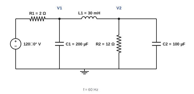
import numpy as np

# Nodal analysis at 60 Hz. Source 120 V (rms, angle 0) through R1 to node 1;
# node 1 to ground: C1; node 1 to node 2: L1; node 2 to ground: R2 in parallel with C2.
f = 60.0
w = 2 * np.pi * f
Vs = 120.0
R1, C1, L1, R2, C2 = 2.0, 200e-6, 30e-3, 12.0, 100e-6
Y = lambda Z: 1 / Z
ZC1, ZL1, ZC2 = 1 / (1j * w * C1), 1j * w * L1, 1 / (1j * w * C2)

# Admittance matrix and current-injection vector (source converted to a Norton equivalent)
G = np.array([[Y(R1) + Y(ZC1) + Y(ZL1), -Y(ZL1)],
              [-Y(ZL1), Y(ZL1) + Y(R2) + Y(ZC2)]])
I = np.array([Vs / R1, 0])
V = np.linalg.solve(G, I)

def polar(z):
    return f"{abs(z):7.2f} at {np.degrees(np.angle(z)):7.2f} deg"

for k, v in enumerate(V, start=1):
    print(f"V{k} = {polar(v)} V")
Is = (Vs - V[0]) / R1
S = Vs * np.conj(Is)
print(f"source current {polar(Is)} A")
print(f"source power P = {S.real:.1f} W, Q = {S.imag:.1f} var, pf = {S.real / abs(S):.3f}")
print(f"power in R2 = {abs(V[1]) ** 2 / R2:.1f} W, in R1 = {abs(Is) ** 2 * R1:.1f} W")

V1 =  105.42 at   -2.88 deg V
V2 =   95.54 at  -61.56 deg V
source current    7.82 at   19.82 deg A
source power P = 883.1 W, Q = -318.3 var, pf = 0.941
power in R2 = 760.7 W, in R1 = 122.4 W

The power balance at the end is an essential check: the real power delivered by the source must equal the sum of the powers in the resistors, because inductors and capacitors absorb no average power. Here 883.1 W = 760.7 W + 122.4 W. The negative reactive power shows that the circuit as a whole is capacitive at 60 Hz.

Mesh analysis

Mesh analysis writes Kirchhoff's voltage law around each mesh of a planar circuit in terms of mesh currents, giving \(\mathbf{Z}\mathbf{I} = \mathbf{V}\), with the sum of impedances around each mesh on the diagonal and the negatives of shared impedances off the diagonal. It is usually the better choice when a circuit has more nodes than meshes, or many voltage sources.

Thévenin and Norton equivalents

Any linear AC circuit seen from two terminals is equivalent, at one frequency, to a voltage source \(V_{th}\) in series with an impedance \(Z_{th}\), or a current source \(I_N = V_{th}/Z_{th}\) in parallel with \(Z_{th}\). \(V_{th}\) is the open-circuit voltage; \(Z_{th}\) is the impedance seen with independent sources turned off (or \(V_{oc}/I_{sc}\), or found with a test source when dependent sources are present).

The equivalent is valid only at the frequency for which it was calculated, because the impedances of inductors and capacitors change with frequency. Within that limit it is extremely useful: it is the basis of maximum power transfer (Lesson 5), of source impedance in power systems (the Thévenin impedance at a bus determines its fault current), and of input and output impedance in electronics.

Superposition and multiple frequencies

Superposition says that the response of a linear circuit to several independent sources is the sum of its responses to each source acting alone. In AC circuits it has a special role: it is the only way to analyze a circuit containing sources at different frequencies, because phasors at different frequencies cannot be added.

The procedure is to analyze the circuit once for each frequency, with the impedances recalculated at that frequency, convert each result to the time domain, and add the time functions. A DC source is simply a source at zero frequency, where inductors are short circuits and capacitors open circuits.

import numpy as np

# v(t) = 10 cos(1000 t) + 5 cos(3000 t + 30 deg) across a series R-L load
R, L = 3.0, 4e-3
parts = [(10.0, 0.0, 1000.0), (5.0, 30.0, 3000.0)]

total_p = 0.0
currents = []
for Vm, ph, w in parts:
    Z = R + 1j * w * L
    I = Vm * np.exp(1j * np.radians(ph)) / Z           # peak phasor at this frequency
    currents.append((abs(I), np.degrees(np.angle(I)), w))
    total_p += 0.5 * abs(I) ** 2 * R
    print(f"w = {w:6.0f} rad/s: Z = {abs(Z):.2f} at {np.degrees(np.angle(Z)):.1f} deg, I = {abs(I):.3f} A at {np.degrees(np.angle(I)):.1f} deg")

# Time-domain check: build i(t) and compute average power and rms directly
t = np.linspace(0, 2 * np.pi / 1000, 200001)
i = sum(Im * np.cos(w * t + np.radians(ph)) for Im, ph, w in currents)
v = sum(Vm * np.cos(w * t + np.radians(ph)) for Vm, ph, w in parts)
print(f"average power: superposition {total_p:.3f} W, time domain {np.mean(v * i):.3f} W")
print(f"rms current: {np.sqrt(np.mean(i ** 2)):.3f} A = sqrt(sum of squares of rms parts) {np.sqrt(sum((Im / np.sqrt(2)) ** 2 for Im, _, _ in currents)):.3f} A")

w =   1000 rad/s: Z = 5.00 at 53.1 deg, I = 2.000 A at -53.1 deg
w =   3000 rad/s: Z = 12.37 at 76.0 deg, I = 0.404 A at -46.0 deg
average power: superposition 6.245 W, time domain 6.245 W
rms current: 1.443 A = sqrt(sum of squares of rms parts) 1.443 A

Two results from this example hold generally. The average power of a sum of sinusoids at different frequencies is the sum of the powers at each frequency, because the cross products average to zero. And the RMS value is the square root of the sum of the squares of the RMS values of the components. These are the foundations of harmonic analysis (Lesson 11).

Op-amp circuits in AC

The ideal op-amp rules (no input current, equal input voltages under negative feedback) apply to phasors just as to DC signals, so op-amp circuits with capacitors are analyzed by replacing resistors with impedances. The inverting amplifier's gain becomes \(-Z_f/Z_i\):

• With a capacitor as \(Z_f\) and a resistor as \(Z_i\): \(H(j\omega) = -1/(j\omega RC)\), an integrator, whose gain falls by a factor of 10 for each decade of frequency.
• With a capacitor as \(Z_i\) and a resistor as \(Z_f\): \(H(j\omega) = -j\omega RC\), a differentiator, whose gain rises with frequency, amplifying noise; practical differentiators add a series resistor to limit high-frequency gain.
• With a resistor in parallel with a capacitor as \(Z_f\): a first-order low-pass filter with gain \(-R_f/R_i\) at low frequency (Lesson 9).

Phasor diagrams as a design tool

A phasor diagram draws the voltages and currents of a circuit as arrows in the complex plane. It shows at a glance which quantities lead or lag, how voltage drops add, and why, for example, the voltage at the end of a long feeder can be lower than or even higher than the source voltage, depending on the power factor of the load. Sketching one before calculating often reveals the shape of the answer, and checking that the calculated phasors close (that KVL and KCL hold graphically) catches sign and angle errors.