
ECON-102 · Lesson 9 of 12 · 29 min
Aggregate demand and aggregate supply
Lessons 5 and 6 explained the long run, in which output is determined by productivity, capital and labor and prices adjust fully. But in the short run the economy can produce more or less than its potential, as recessions and booms show. To analyze these fluctuations, economists use the model of aggregate demand and aggregate supply (AD-AS). It looks like the supply and demand diagram of ECON-101, but the axes measure the economy as a whole: real GDP on the horizontal axis and the overall price level on the vertical axis. The curves have different explanations from those of a single market, and confusing the two is a common mistake. This lesson builds the model, uses it to analyze demand shocks and supply shocks, and introduces the spending multiplier.
Aggregate demand
Aggregate demand (AD) is the total quantity of final goods and services that households, firms, governments and foreigners want to buy at each price level: \( C + I + G + NX \). The AD curve slopes downward, but not for the reason a single demand curve does. In a single market, a higher price makes buyers switch to other goods; for the whole economy there is nothing else to switch to. Instead, three effects explain the slope. The wealth effect: a higher price level reduces the real value of money and other nominal assets, so households feel poorer and spend less. The interest rate effect: a higher price level raises the demand for money to make transactions, which tends to push up interest rates and reduce investment and interest-sensitive consumption; in modern practice, the central bank also tends to raise interest rates when prices rise faster. The exchange rate effect: higher domestic prices make domestic goods more expensive relative to foreign goods, reducing net exports.
The AD curve shifts when spending changes at any given price level. It shifts right when consumer or business confidence rises, when household wealth rises because of higher stock or house prices, when the government increases purchases or cuts taxes, when the central bank lowers interest rates, when foreign incomes rise and boost exports, or when the currency depreciates. It shifts left in the opposite cases. Many of the most important events in macroeconomics, such as the collapse of investment and consumption in 2008–2009, or the surge in spending supported by fiscal programs and low rates in 2021, are shifts in aggregate demand.
Aggregate supply in the long run
The long-run aggregate supply (LRAS) curve is vertical at potential output. In the long run, the quantity of output the economy can produce depends on labor, capital, natural resources and technology, as lesson 5 explained, not on the price level. If all prices and wages doubled, real output would be unchanged. The LRAS curve shifts right when the labor force grows, when capital accumulates, when education improves or when technology advances, and it shifts left if productive capacity is destroyed, for example by a natural disaster or a war.
Aggregate supply in the short run
The short-run aggregate supply (SRAS) curve slopes upward: in the short run, a higher price level is associated with more output. The reason is that some prices and costs are sticky. Wages are often set by contracts or adjusted only once a year; many firms change prices infrequently because of menu costs or concern about customer relations; and workers and firms may not immediately recognize that a rise in their own prices reflects a general rise in prices. If the price level rises unexpectedly while wages are fixed, firms' profit margins improve and they expand output. If prices fall unexpectedly, margins shrink and firms cut production and employment.
The SRAS curve shifts when production costs change at any given price level. It shifts left (up) when wages rise, when the prices of key inputs such as oil rise, when expected inflation rises (because workers and firms build expected price increases into wages and prices), or when supply chains are disrupted. It shifts right when input costs fall or productivity improves. A leftward shift of SRAS caused by a sudden rise in costs is called an adverse supply shock.
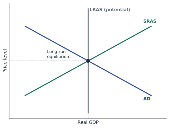
The economy is in long-run equilibrium when AD intersects SRAS at a point on the LRAS curve: output equals potential, and the price level is what people expected, so there is no pressure on wages and prices to change faster than expected. In the short run, AD and SRAS can intersect to the left of LRAS (a recessionary gap) or to the right (an inflationary gap). Over time, wages and prices adjust and the economy moves back toward potential, though this adjustment may be slow, which is why policy can play a stabilizing role.
A demand shock
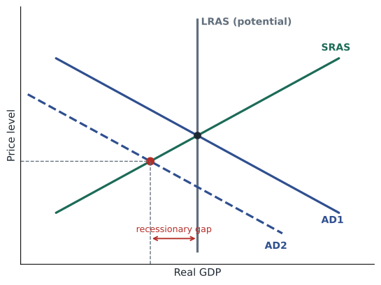
Suppose a fall in business confidence reduces investment, shifting AD to the left. In the short run, the economy moves down along SRAS: output falls below potential, unemployment rises, and inflation falls. The economy has a recessionary gap. What happens next? With output below potential and unemployment high, wage growth slows and firms cut prices or raise them more slowly. Lower costs gradually shift SRAS to the right, returning output to potential at a lower price level (or, with ongoing inflation, a lower inflation rate). This self-correcting process may take years, however, and in the meantime unemployment imposes real costs. Alternatively, the central bank can cut interest rates or the government can raise spending to shift AD back to the right, speeding recovery. A positive demand shock works in reverse: output rises above potential, unemployment falls below the natural rate, and inflation rises, until rising costs shift SRAS left or policy tightens.
Worked problem
Analyzing a demand shock
An economy is at potential output with inflation at 2 %. A sharp fall in exports reduces aggregate demand. Describe the short-run effects, the long-run self-correction and a policy response.
Show solution
- Short run: AD shifts left; output falls below potential, unemployment rises and inflation falls below 2 %.
- Self-correction: slack slows wage and price growth, shifting SRAS right until output returns to potential.
- Policy: the central bank can cut its policy rate (lesson 8) or the government can raise spending or cut taxes (lesson 10), shifting AD back to the right.
- A cheaper currency, as the central bank cuts rates, also helps restore net exports.
Answer: A demand shock moves output and inflation in the same direction, so stabilization policy faces no conflict: stimulus helps both employment and inflation return to normal.
A supply shock
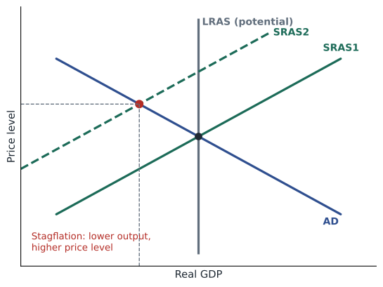
Now suppose a sharp rise in oil prices raises production costs across the economy, shifting SRAS to the left. In the short run, output falls and the price level rises: the economy suffers stagflation, a combination of stagnation and inflation. Supply shocks are much harder for policymakers than demand shocks, because output and inflation move in opposite directions. If the central bank cuts interest rates to support output, it adds to inflation; if it raises rates to fight inflation, it deepens the slowdown. If it does nothing, the economy may adjust as the shock fades or as wages adjust, but inflation will be above target for a time.
The 1970s provide the classic example. Oil prices quadrupled in 1973–1974 and rose sharply again in 1979–1980, contributing to high inflation and recessions in Canada, the United States and most other oil-importing countries. Because central banks had accommodated earlier inflation, expectations had become unanchored, and the shocks set off a wage-price spiral. Bringing inflation down required very high interest rates in the early 1980s, which caused deep recessions. The lesson that central banks drew was that anchored inflation expectations make supply shocks much less costly, because a one-time rise in prices does not turn into persistent inflation.
The 2026 oil shock posed this dilemma again. Higher gasoline prices pushed headline CPI inflation to 3.7 % in September 2026, while payroll growth slowed sharply. Because inflation had been above the Fed's 2 % target for more than five years, the FOMC worried that expectations could drift upward and raised its target range in September. The United States is now a net exporter of petroleum, so higher oil prices raise incomes in producing states such as Texas and North Dakota, but most consumers and many businesses lose, and the overall effect on growth is still negative in the short run.
Inflation expectations and the shifting SRAS
Expected inflation shifts the SRAS curve. If workers and firms expect 2 % inflation, wages and prices rise by about 2 % a year even with output at potential. If they come to expect 5 %, they build 5 % into contracts, and the SRAS curve shifts up faster. This is why central banks watch surveys of expected inflation and financial market measures closely. When expectations are anchored, temporary shocks fade; when they are not, inflation becomes self-perpetuating. Lesson 12 develops this idea with the Phillips curve.
The spending multiplier
Changes in spending have effects larger than their initial size, because one person's spending is another's income. If the government spends 100 million dollars more on infrastructure, construction workers and firms earn 100 million more. They spend part of it, say 60 %, on consumer goods, which becomes income for others, who spend 60 % of that, and so on. The marginal propensity to consume (MPC) is the fraction of an extra dollar of disposable income that households spend. In the simplest model, with no taxes or imports, the total increase in spending is \( 1 / (1 - MPC) \) times the initial change.
In real economies, part of each extra dollar of income goes to taxes and part is spent on imports, which leak out of the domestic spending stream. If \( t \) is the marginal tax rate and \( m \) the marginal propensity to import (the share of each extra dollar of income spent on imports), the multiplier becomes smaller.
Worked problem
Calculating the multiplier
The MPC is 0.8, the marginal tax rate 0.3 and the marginal propensity to import 0.25. Calculate the simple multiplier and the multiplier with taxes and imports. By how much does GDP rise if government purchases increase by 10 billion dollars, assuming no change in interest rates?
Show solution
- Simple multiplier = 1 ÷ (1 − 0.8) = 5.
- With taxes and imports: 1 ÷ (1 − 0.8 × 0.7 + 0.25) = 1 ÷ (1 − 0.56 + 0.25) = 1 ÷ 0.69 ≈ 1.45.
- Change in GDP ≈ 1.45 × 10 = 14.5 billion dollars.
Answer: Taxes and imports shrink the multiplier from 5 to about 1.45. In an open economy with high import shares, much of the stimulus leaks abroad.
# Multiplier rounds: initial spending, then successive rounds of induced consumption
mpc, t, m = 0.8, 0.3, 0.25
induced = mpc * (1 - t) - m        # extra domestic spending per extra dollar of income
dG = 10.0                          # billions
round_spend, total = dG, 0.0
for r in range(1, 31):
    total += round_spend
    if r in (1, 2, 3, 5, 30):
        print(f"after round {r:2d}: cumulative GDP change {total:6.2f} billion")
    round_spend *= induced
print(f"formula: 1 / (1 - MPC(1 - t) + m) = {1 / (1 - mpc * (1 - t) + m):.3f}")after round 1: cumulative GDP change 10.00 billion after round 2: cumulative GDP change 13.10 billion after round 3: cumulative GDP change 14.06 billion after round 5: cumulative GDP change 14.45 billion after round 30: cumulative GDP change 14.49 billion formula: 1 / (1 - MPC(1 - t) + m) = 1.449
Real-world multipliers are smaller and less certain than this formula suggests, for several reasons. When the economy is near full employment, extra spending mainly raises prices rather than output. The central bank may raise interest rates to offset fiscal stimulus, crowding out investment. Households may save temporary tax cuts rather than spend them, especially if they expect future tax increases. And the multiplier depends on the type of spending: transfers to low-income households, who spend most of what they receive, tend to have larger effects than tax cuts for high-income households. Empirical estimates of government spending multipliers range widely, from below 0.5 to above 2, with larger values found in deep recessions when interest rates are at their lower bound. Lesson 10 discusses these debates.
| Shock | Curve that shifts | Short-run output | Short-run price level | Policy dilemma? |
|---|---|---|---|---|
| Fall in consumer or business confidence | AD left | Falls | Falls | No: stimulus helps both |
| Fiscal stimulus or rate cut | AD right | Rises | Rises | Risk of overheating near potential |
| Oil price spike | SRAS left | Falls | Rises | Yes: stagflation |
| Productivity improvement | SRAS and LRAS right | Rises | Falls | No |
| Rise in expected inflation | SRAS left | Falls | Rises | Yes |
Common mistakes
MistakeThe AD curve slopes down because buyers switch to other goods.
InsteadIt slopes down because of wealth, interest rate and exchange rate effects; for the whole economy there are no substitutes.
MistakeSupply shocks and demand shocks call for the same response.
InsteadDemand shocks move output and inflation together; supply shocks move them in opposite directions, creating a dilemma.
MistakeThe multiplier is always 1 ÷ (1 − MPC).
InsteadTaxes, imports, crowding out and capacity limits make real multipliers much smaller.
MistakeIn the long run, more demand means more output.
InsteadIn the long run output returns to potential; extra demand raises the price level.
MistakeA one-time oil price rise must cause lasting inflation.
InsteadWith anchored expectations, it raises the price level once and inflation returns toward target.
Summary and key terms
- The AD-AS model analyses short-run fluctuations in real GDP and the price level.
- AD slopes downward because of wealth, interest rate and exchange rate effects; it shifts with confidence, wealth, fiscal and monetary policy and foreign demand.
- LRAS is vertical at potential output; SRAS slopes upward because wages and some prices are sticky.
- Demand shocks move output and inflation in the same direction; the economy self-corrects slowly, and policy can speed recovery.
- Supply shocks cause stagflation and create a policy dilemma; anchored expectations limit their damage.
- Expected inflation shifts SRAS, so credibility matters.
- The spending multiplier amplifies changes in spending but is reduced by taxes, imports, crowding out and capacity limits.
- Aggregate demand (AD)
- Total spending on final goods and services at each price level.
- Short-run aggregate supply (SRAS)
- The relationship between the price level and output when some prices and wages are sticky.
- Long-run aggregate supply (LRAS)
- A vertical line at potential output.
- Recessionary gap
- Output below potential.
- Inflationary gap
- Output above potential.
- Demand shock
- An event that shifts aggregate demand.
- Supply shock
- An event that shifts aggregate supply, such as a change in input costs.
- Stagflation
- Falling output combined with rising prices.
- Marginal propensity to consume (MPC)
- The share of an extra dollar of disposable income that is spent.
- Spending multiplier
- The ratio of the total change in GDP to an initial change in spending.
Practice problems
Work each problem on paper first, then reveal the answer to check.
Give three reasons the AD curve slopes downward.
Show answer
Wealth effect, interest rate effect, exchange rate effect.
Why is LRAS vertical?
Show answer
Long-run output depends on resources and technology, not the price level.
What happens in the short run when AD shifts right at potential?
Show answer
Output rises above potential and the price level rises.
Describe the self-correction from a recessionary gap.
Show answer
Slack slows wage and price growth, shifting SRAS right until output returns to potential.
Why is a supply shock harder for policy than a demand shock?
Show answer
It raises prices while lowering output, so stimulus worsens inflation and tightening worsens output.
MPC 0.75, no taxes or imports. Multiplier?
Show answer
4.
MPC 0.9, tax rate 0.25, import propensity 0.3. Multiplier?
Show answer
1 ÷ (1 − 0.675 + 0.3) = 1.6.
Why might a temporary tax cut have a small multiplier?
Show answer
Households may save it, especially if they expect future tax increases.
How do expectations affect SRAS?
Show answer
Higher expected inflation shifts SRAS up as wages and prices are set higher.
Portfolio task: identify a recent shock to your economy and classify it as a demand or supply shock, explaining its effect with an AD-AS diagram.
Show answer
Answers vary; should correctly identify which curve shifts.
Lesson quiz · 5 questions
Score 60% or more to complete this lesson.
Create a free account to save your progress, take quizzes and earn a certificate.