
ECON-102 · Lesson 12 of 12 · 29 min
Macroeconomic policy debates and capstone: analyzing an economic briefing
The previous lessons built a toolkit: measures of output, prices and unemployment; models of long-run growth, saving and investment; money, banking and central banks; aggregate demand and supply; fiscal policy and debt; and the open economy. This final lesson uses that toolkit to examine the main debates in macroeconomic policy, where reasonable economists disagree because the evidence is incomplete or because they weigh outcomes differently. It then guides you through a capstone: analyzing a current economic briefing and writing a balanced policy assessment. The aim is not to tell you what to conclude, but to help you reason clearly, use evidence and recognize the value judgments involved.
The Phillips curve: is there a trade-off between inflation and unemployment?
In 1958 the New Zealand-born economist A. W. Phillips showed that, in British data, years of low unemployment tended to be years of rapid wage growth. Economists soon found a similar negative relationship between unemployment and price inflation, and in the 1960s many believed that policymakers could choose a point on this Phillips curve, accepting somewhat higher inflation in exchange for permanently lower unemployment. Milton Friedman and Edmund Phelps argued that this trade-off would not last. If policymakers tried to hold unemployment below its natural rate, workers and firms would come to expect higher inflation and build it into wages and prices, shifting the short-run Phillips curve up. In the long run, unemployment would return to the natural rate, with higher inflation. The long-run Phillips curve is vertical at the natural rate of unemployment. The stagflation of the 1970s confirmed this prediction dramatically.
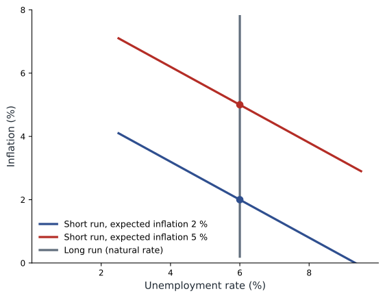
The modern expectations-augmented Phillips curve says that inflation equals expected inflation, minus a term that rises when unemployment is below its natural rate, plus supply shocks (\( \varepsilon \)). When expectations are anchored at the 2 % target, inflation varies with slack and supply shocks around 2 %. Two puzzles have dominated recent debate. Before 2020, the Phillips curve appeared to have become very flat: unemployment fell to historic lows without much rise in inflation, leading some to argue that slack no longer mattered much. Then in 2021–2022 inflation surged as labor markets became extremely tight, suggesting the curve becomes steep when the economy runs very hot, with job vacancies far exceeding unemployed workers. Many economists now think the relationship is non-linear: flat in normal times, steep when the economy is overheated.
Worked problem
The expectations-augmented Phillips curve
Expected inflation is 2 %, the natural rate of unemployment is 6 %, and β = 0.5. Find inflation when unemployment is 5 % with no supply shock, and when unemployment is 6.5 % with an oil shock adding 1.5 points.
Show solution
- Unemployment 5 %: π = 2 − 0.5 × (5 − 6) = 2.5 %.
- Unemployment 6.5 % with shock: π = 2 − 0.5 × 0.5 + 1.5 = 3.25 %.
Answer: Tight labor markets add half a point of inflation. In the second case, inflation is above target despite slack, because of the supply shock: the stagflation dilemma in numbers.
Rules versus discretion
Should central banks follow rules, such as the Taylor rule of lesson 8, or use discretion? Advocates of rules argue that they make policy predictable, protect central banks from political pressure, and avoid the temptation to stimulate the economy at the cost of future inflation, a problem known as time inconsistency. Advocates of discretion argue that no simple rule can anticipate every situation, such as a pandemic, a financial crisis or a supply shock, and that judgment is needed. Inflation targeting is often described as constrained discretion: a clear goal, transparent communication and accountability, combined with flexibility in how and when to act. Most economists support this middle ground, but they debate how much weight to give rules in communication and how quickly central banks should respond to deviations from target.
Should central banks look through supply shocks?
The 2021–2023 inflation and the 2026 oil shock revived a classic question. Standard theory says that central banks should look through temporary supply shocks, because raising rates cannot increase the supply of oil or semiconductors and would only add a recession to the inflation. But the 2021–2022 experience showed that what looks temporary can persist, especially when supply shocks hit an economy where demand is already strong, and that inflation expectations may not stay anchored indefinitely after years above target. One school argues that central banks should respond only if core inflation and expectations show signs of spillover; another argues that after a long period of above-target inflation, credibility requires a firmer response even to supply shocks.
In autumn 2026 the Federal Reserve chose to respond, raising its target range to 3.75–4.00 % with core PCE inflation above 3 % after five years above target. Critics on one side argued that the energy shock was temporary and that payroll growth had slowed sharply; critics on the other side argued that the Fed had been too slow to act in 2021 and needed to protect its credibility.
How much government debt is too much?
Lesson 10 showed that debt sustainability depends on the gap between interest rates and growth and on the primary balance. During the 2010s, when interest rates were below growth rates, some economists, such as Olivier Blanchard, argued that the fiscal costs of debt were lower than commonly believed and that governments could borrow more to invest. Since 2022, higher interest rates have raised debt service costs, and others argue that rising debt ratios, especially in the United States, create risks of higher interest rates, reduced room to respond to future crises and difficult choices for future taxpayers. Points of agreement include that debt incurred to fund productive investment is easier to justify than debt for current spending, that credible medium-term fiscal plans reduce risks, and that aging populations will raise spending pressures. Disagreement centers on how fast to reduce deficits, through taxes or spending, and how much weight to give the needs of current versus future generations.
Inequality, climate and technology
Several newer debates cross into macroeconomics. Does inequality affect macroeconomic outcomes? Some research suggests that high inequality can weaken demand, because high-income households save more of their income, and can contribute to financial instability through household borrowing, while other research emphasizes incentives and growth. Climate change raises questions about how physical damage, carbon pricing and the transition to low-carbon energy affect growth, inflation and financial stability. Central banks, including the Bank of Canada, have studied climate scenarios, while debating how far their mandates extend; the US Federal Reserve withdrew from the international Network for Greening the Financial System in 2025.
In the United States, climate policy has relied mainly on tax credits and regulation rather than carbon pricing; the 2022 Inflation Reduction Act expanded clean energy tax credits, many of which were scaled back or phased out by the July 2025 reconciliation law. Economists debate how best to reduce emissions at the lowest economic cost: most favor carbon pricing as the most efficient tool, while others emphasize regulations, subsidies and investment, which are more politically popular but often costlier per metric ton of emissions avoided.
Finally, artificial intelligence raises macroeconomic questions discussed in lesson 5: will it raise productivity growth enough to ease fiscal pressures and raise wages, or will it displace workers faster than new jobs appear? A rapid investment boom in data centers and chips has already added to demand and to electricity prices in some regions. The answers remain uncertain, which is itself an important lesson: policy must be made under uncertainty, and good policy frameworks are robust to a range of possible outcomes.
| Debate | One view | Another view | What evidence helps decide |
|---|---|---|---|
| Response to supply shocks | Look through temporary shocks | Act to protect credibility after long overshoots | Core inflation, expectations surveys, wage growth |
| Size of fiscal multipliers | Large in recessions | Small because of crowding out and expectations | Natural experiments, state of the economy |
| Government debt | Manageable while growth exceeds interest rates | Rising debt creates risks and burdens | Interest-growth gap, market reactions, aging costs |
| Rules versus discretion | Rules give predictability | Discretion handles unusual shocks | Historical performance of rule-like and discretionary policy |
| Climate policy | Carbon pricing is cheapest | Subsidies and regulation are more feasible | Cost per metric ton avoided, political durability |
Capstone: analyzing an economic briefing
Your capstone task is to analyze a current economic briefing and write a balanced policy assessment of about 1,200 words. Choose a recent official document, such as a central bank monetary policy report or rate announcement, a government budget or fiscal update, or an assessment by an independent fiscal or statistical agency. Work through the following steps.
Step 1, gather the indicators. Record the latest real GDP growth rate, output gap estimate, unemployment rate, participation rate, headline and core inflation, the policy interest rate, the government budget balance and debt ratio, and the exchange rate. Note the date and source of each figure, and whether it is preliminary.
Step 2, diagnose the state of the economy. Is output above or below potential? Is inflation above or below target, and is it driven by demand, supply shocks or expectations? Use the AD-AS model to identify which curves have shifted recently and why. Use Okun's law and the Phillips curve to check whether unemployment and inflation are consistent with your view of the output gap.
Step 3, evaluate the policy stance. Calculate the real policy interest rate using the Fisher equation and compare it with estimates of the neutral rate. Compute a Taylor rule benchmark under at least two sets of assumptions. Assess fiscal policy using the cyclically adjusted balance where available, and the debt dynamics equation to judge sustainability.
Step 4, consider the risks. Identify the main upside and downside risks, such as energy prices, trade policy, financial conditions, housing and global growth, and explain how each would affect output and inflation.
Step 5, present the debate. Set out the strongest case for at least two different policy options, such as holding, raising or cutting the policy rate, or tightening or loosening fiscal policy. Distinguish clearly between positive claims and value judgments. Conclude with your own recommendation, explaining which evidence and values led you to it.
Worked problem
A worked briefing snapshot: United States, October 2026
Using the figures reported in this course, assess the Fed's stance. Data: unemployment 4.2 % (natural rate assumed 4.2 %); headline CPI inflation 3.7 %; core PCE inflation about 3.3 %; federal funds target 3.75–4.00 %; median long-run neutral nominal rate about 3 %.
Show solution
- Okun's law: unemployment near the assumed natural rate suggests an output gap near zero.
- Real policy rate using core PCE inflation: 3.875 − 3.3 ≈ 0.6 %, close to a neutral real rate of about 1 %, so policy is roughly neutral.
- Taylor rule (r* = 1 %, gap 0): 1 + 3.3 + 0.5 × 1.3 = 4.95 %.
- Diagnosis: output near potential, inflation above target partly because of energy, and payroll growth slowing.
Answer: The Taylor rule points to a rate above the current range, supporting the September increase; but slowing job growth and the temporary nature of an oil shock argue for caution about further increases. Reasonable analysts disagree.
# Briefing dashboard: real rates, Okun gap and Taylor benchmarks (figures as reported, Oct 2026)
data = {
    'Canada': dict(policy=2.25, core=1.9, headline=3.1, unemp=6.5, u_star=6.0, r_star=0.75),
    'United States': dict(policy=3.875, core=3.3, headline=3.7, unemp=4.2, u_star=4.2, r_star=1.0),
}
okun, target = 0.5, 2.0
for country, d in data.items():
    gap = (d['u_star'] - d['unemp']) / okun
    real = d['policy'] - d['core']
    t_core = d['r_star'] + d['core'] + 0.5 * (d['core'] - target) + 0.5 * gap
    t_head = d['r_star'] + d['headline'] + 0.5 * (d['headline'] - target) + 0.5 * gap
    print(f"{country}: output gap ~{gap:+.1f} %, real policy rate {real:.2f} %, "
f"Taylor (core) {t_core:.2f} %, Taylor (headline) {t_head:.2f} %, actual {d['policy']:.2f} %")Canada: output gap ~-1.0 %, real policy rate 0.35 %, Taylor (core) 2.10 %, Taylor (headline) 3.90 %, actual 2.25 % United States: output gap ~+0.0 %, real policy rate 0.58 %, Taylor (core) 4.95 %, Taylor (headline) 5.55 %, actual 3.88 %
Note how sensitive the conclusions are to assumptions about the natural rate of unemployment, the neutral interest rate and the right measure of inflation. That sensitivity is not a flaw in the analysis; it is the reality policymakers face. A strong briefing states its assumptions openly, tests alternatives and explains why one judgment is more persuasive than another.
Writing a balanced assessment
Good economic writing for policy audiences shares several features. It starts with the main conclusion, then supports it with evidence. It uses a few well-chosen numbers rather than a flood of data, and it always gives dates and sources. It distinguishes facts from forecasts and forecasts from recommendations. It presents opposing views fairly, in their strongest form, rather than as straw men. It quantifies uncertainty where possible, for example by describing what would change the recommendation. And it avoids jargon or explains it. These habits will serve you well whether you work in business, government, journalism or finance, or simply want to be an informed citizen.
Common mistakes
MistakeThere is a permanent trade-off between inflation and unemployment.
InsteadThe short-run trade-off depends on expectations; in the long run unemployment returns to the natural rate.
MistakeEvery inflation increase requires higher interest rates.
InsteadTemporary supply shocks may be looked through if expectations stay anchored; persistent pressures require action.
MistakeA Taylor rule gives the correct policy rate.
InsteadIt is a benchmark sensitive to unobservable assumptions such as the neutral rate and output gap.
MistakeEconomic debates are purely technical.
InsteadMany involve value judgments about inflation versus unemployment, or present versus future generations.
MistakeOne indicator is enough to judge the economy.
InsteadCombine output, labor, inflation, financial and fiscal indicators and check their consistency.
Summary and key terms
- The expectations-augmented Phillips curve links inflation to expected inflation, slack and supply shocks; the long-run curve is vertical.
- The Phillips curve appears flat in normal times and steep when the economy overheats.
- Inflation targeting is constrained discretion, combining a clear goal with flexibility.
- Central banks debate whether to look through supply shocks or act to protect credibility.
- Debt debates hinge on the interest-growth gap, the purpose of borrowing and intergenerational values.
- Inequality, climate and AI are increasingly important for macroeconomic policy.
- A strong briefing gathers indicators, diagnoses the economy, evaluates the policy stance, weighs risks and presents opposing views fairly.
- Phillips curve
- A relationship between unemployment and inflation.
- Expectations-augmented Phillips curve
- A Phillips curve in which expected inflation shifts the short-run trade-off.
- Long-run Phillips curve
- A vertical line at the natural rate of unemployment.
- Time inconsistency
- The temptation to depart from earlier commitments once others have acted on them.
- Constrained discretion
- Policy with a clear goal and accountability but flexibility in implementation.
- Look through
- To leave policy unchanged in response to a temporary shock.
- Real policy rate
- The policy interest rate minus inflation or expected inflation.
- Policy stance
- Whether policy is stimulating, neutral or restraining the economy.
- Upside risk
- A possibility that outcomes will be stronger or higher than forecast.
- Downside risk
- A possibility that outcomes will be weaker or lower than forecast.
Practice problems
Work each problem on paper first, then reveal the answer to check.
Why is the long-run Phillips curve vertical?
Show answer
Expectations adjust, so unemployment returns to the natural rate whatever the inflation rate.
π^e = 2 %, u* = 5 %, u = 4 %, β = 0.4. Find inflation.
Show answer
2.4 %.
What caused the stagflation of the 1970s?
Show answer
Oil supply shocks combined with unanchored inflation expectations.
What is time inconsistency?
Show answer
The temptation to break a promise, such as low inflation, once people have acted on it.
Give one argument for looking through an oil price shock.
Show answer
Rate increases cannot raise oil supply and would add a recession; the shock may fade.
Give one argument against.
Show answer
After years above target, expectations may rise and credibility may need protecting.
Policy rate 3 %, expected inflation 2.5 %. Real policy rate?
Show answer
0.5 %.
Why do assumptions matter in a Taylor rule assessment?
Show answer
The neutral rate and output gap are unobservable and change the answer.
Name two features of good policy writing.
Show answer
Conclusion first, dated sources, facts separated from forecasts, fair presentation of opposing views.
Capstone: write a 1,200-word assessment of your country's current monetary and fiscal stance using the five steps.
Show answer
Answers vary; should use current data, models and balanced arguments.
Lesson quiz · 5 questions
Score 60% or more to complete this lesson.
Create a free account to save your progress, take quizzes and earn a certificate.