
ECON-102 · Lesson 10 of 12 · 28 min
Fiscal policy, deficits and debt
Fiscal policy is the use of government spending and taxation to influence the economy. Governments spend on health care, education, defense, infrastructure and income support, and they raise revenue through income taxes, sales taxes, payroll contributions, corporate taxes, tariffs and other levies. When spending exceeds revenue, the government runs a deficit and borrows, adding to its debt. Fiscal policy affects the economy in the short run through aggregate demand and in the long run through saving, investment and incentives. This lesson explains how budgets work, the difference between automatic stabilizers and discretionary policy, the evidence on fiscal multipliers, and the arithmetic of government debt.
Government budgets
The United States is a federation in which the federal government is responsible for defense, Social Security, Medicare, much of Medicaid funding, veterans' benefits and interest on federal debt, while states and localities fund most education, policing and infrastructure. Most states are required by their constitutions to balance their operating budgets, so most deficit spending occurs at the federal level. The federal fiscal year runs from 1 October to 30 September. The President proposes a budget, but Congress controls spending through appropriations bills, and much spending, including Social Security and Medicare, is mandatory under existing law. The nonpartisan Congressional Budget Office (CBO) produces baseline projections and estimates the cost of legislation. A statutory debt limit caps total federal borrowing; Congress raised it by 5 trillion dollars in the reconciliation law enacted in July 2025.
The budget balance is revenue minus spending. A deficit adds to the stock of government debt; a surplus reduces it. Economists distinguish the primary balance, which excludes interest payments on the debt, from the total balance. The primary balance shows whether current programs are paid for by current revenue; the total balance adds the cost of servicing past borrowing. They also distinguish gross debt from net debt, which subtracts financial assets such as pension fund holdings.
| Measure | Federal government, fiscal year 2026 | Source |
|---|---|---|
| Deficit | About 2.0 trillion dollars (about 6.2 % of GDP) | CBO monthly budget review, October 2026 |
| Debt held by the public | About 32.4 trillion dollars, roughly 100 % of GDP | CBO |
| Net interest | More than 1 trillion dollars, second only to Social Security | CBO |
| Projected debt in 2036 | About 120 % of GDP | CBO Budget and Economic Outlook, February 2026 |
US federal debt held by the public has risen from about 35 % of GDP in 2007 to about 100 % in 2026, driven by the 2008–2009 recession, the pandemic response, tax cuts, and rising spending on Social Security, Medicare and interest as the population ages. The July 2025 reconciliation law extended the individual income tax cuts first enacted in 2017 and added other tax and spending changes, which CBO estimated would add several trillion dollars to deficits over ten years. Tariff revenue rose sharply in 2025, but in February 2026 the Supreme Court ruled that tariffs imposed under emergency powers were unlawful, and the government refunded about 130 billion dollars of them in fiscal year 2026.
Automatic stabilizers
Some parts of the budget change automatically with the business cycle. When the economy weakens, incomes and profits fall, so income and corporate tax revenue falls; spending on unemployment benefits and income-tested programs rises. The deficit widens without any new decision, supporting household incomes and aggregate demand. When the economy booms, the reverse happens. These automatic stabilizers dampen fluctuations, acting quickly and without the political delays of new legislation. Because of them, the actual budget balance is a misleading guide to the stance of fiscal policy. Economists estimate the cyclically adjusted (or structural) balance: what the balance would be if the economy were at potential output. A deficit that persists even at full employment is a structural deficit.
Worked problem
Cyclically adjusted balance
A government has a deficit of 3 % of GDP. The output gap is −2 %, and each point of negative output gap widens the deficit by about 0.5 % of GDP through automatic stabilizers. What is the cyclically adjusted balance?
Show solution
- Cyclical component = 0.5 × 2 = 1 % of GDP of deficit.
- Cyclically adjusted deficit = 3 − 1 = 2 % of GDP.
Answer: Two thirds of the deficit is structural: it would remain even if the economy returned to potential.
Discretionary fiscal policy
Discretionary fiscal policy means deliberate changes in spending or tax laws to stabilize the economy. In a recession, the government can raise spending, cut taxes or increase transfers to boost aggregate demand. In a boom, it can do the opposite. Both countries made very large discretionary moves during the pandemic: programs such as wage subsidies, emergency income benefits, enhanced unemployment benefits and direct payments to households pushed deficits to around 15 % of GDP in 2020 in both countries, the largest since the Second World War. These programs prevented a collapse in household incomes, and household saving actually rose; they also contributed, along with supply disruptions and low interest rates, to the inflation of 2021–2022.
Discretionary policy faces several problems. The first is lags. The recognition lag is the time needed to realize that a downturn has begun; the decision lag is the time needed to design and pass legislation; and the implementation lag is the time before spending reaches the economy. Infrastructure projects can take years to start, by which time the recession may be over. Hence economists often recommend that stimulus be timely, targeted and temporary: delivered quickly, aimed at households likely to spend it, and withdrawn as the economy recovers. The second problem is interaction with monetary policy: if the economy is near capacity, the central bank may raise interest rates to offset fiscal stimulus, reducing its effect. The third is political: it is easier to cut taxes and raise spending in bad times than to reverse them in good times, which tends to produce persistent deficits.
How big are fiscal multipliers?
Lesson 9 derived a simple spending multiplier. Measuring real-world multipliers is difficult, because fiscal policy often responds to economic conditions, so researchers use natural experiments, such as military build-ups driven by wars or regional differences in federal spending. Many studies find government spending multipliers of roughly 0.5 to 1.5 in normal times, with larger effects, possibly above 1.5, in deep recessions when interest rates are at their lower bound and there is much slack. Tax multipliers vary with the type of tax and its permanence. Transfers to lower-income and liquidity-constrained households tend to be spent quickly, while temporary tax cuts for higher-income households are more often saved.
There is genuine disagreement. Some economists argue that multipliers are often below one, because government spending crowds out private spending, households anticipate future taxes (an argument known as Ricardian equivalence, after the economist David Ricardo), and high debt raises interest rates and uncertainty. Others argue that in recessions, with idle resources, fiscal stimulus can raise output by more than its cost and may even improve long-run outcomes by preventing hysteresis. The evidence suggests both camps are right in different circumstances: the effect of fiscal policy depends heavily on the state of the economy, the response of the central bank and how the policy is designed.
The arithmetic of public debt
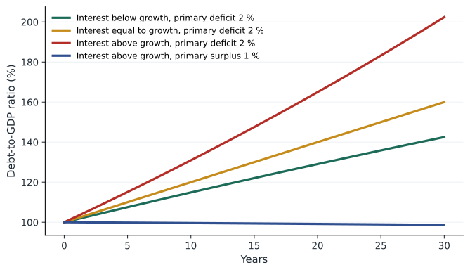
What matters for sustainability is not the dollar size of the debt but the ratio of debt to GDP, which measures the debt relative to the economy's capacity to service it. The change in the debt ratio depends on three things: the primary balance, the interest rate on the debt (\( r \)) and the growth rate of nominal GDP (\( g \)). If the interest rate exceeds the growth rate, the debt ratio tends to rise unless the government runs a primary surplus; if growth exceeds the interest rate, the ratio can fall even with a modest primary deficit.
Here \( d \) is the debt-to-GDP ratio and \( pb \) the primary balance as a share of GDP (positive for a surplus). This simple equation explains much of the history of public debt. After the Second World War, both Canada and the United States reduced very high debt ratios, not mainly by repaying debt but by growing faster than the interest rate, helped at times by inflation. In the 1990s Canada faced a debt crisis: high interest rates and slow growth pushed federal debt above 65 % of GDP, and the 1995 budget's deep spending cuts, followed by a decade of surpluses and strong growth, brought it down to about 30 % by 2008. In the 2010s, very low interest rates made debt cheap to carry, leading some economists to argue that governments could borrow more safely. Since 2022, higher interest rates have raised debt service costs sharply.
Worked problem
Debt dynamics
A government's debt is 100 % of GDP. Nominal GDP grows 4 % a year and the average interest rate on debt is 3.5 %. It runs a primary deficit of 2 % of GDP. What happens to the debt ratio this year? What primary balance would stabilize it?
Show solution
- (r − g) d = (0.035 − 0.04) × 100 = −0.5 points.
- Primary deficit adds 2 points: Δd ≈ −0.5 + 2 = +1.5 points.
- To stabilize: pb = (r − g) d = −0.5, a primary deficit of 0.5 % of GDP.
Answer: The debt ratio rises 1.5 points to about 101.5 %. Because growth exceeds the interest rate, a small primary deficit of 0.5 % of GDP would hold it steady; a larger one makes it rise.
# Debt-to-GDP dynamics under different interest-growth gaps
def path(d0, r, g, pb, years=30):
    d = d0
    out = [d]
    for _ in range(years):
        d = d * (1 + r) / (1 + g) - pb   # exact version of the approximation
        out.append(d)
    return out

scenarios = {
    "r < g, primary deficit 2 %": (100, 0.035, 0.04, -2.0),
    "r = g, primary deficit 2 %": (100, 0.040, 0.04, -2.0),
    "r > g, primary deficit 2 %": (100, 0.050, 0.04, -2.0),
    "r > g, primary surplus 1 %": (100, 0.050, 0.04, 1.0),
}
for name, (d0, r, g, pb) in scenarios.items():
    p = path(d0, r, g, pb)
print(f"{name:28s} year 10 {p[10]:6.1f} % year 20 {p[20]:6.1f} % year 30 {p[30]:6.1f} %")r < g, primary deficit 2 % year 10 114.9 % year 20 129.0 % year 30 142.5 % r = g, primary deficit 2 % year 10 120.0 % year 20 140.0 % year 30 160.0 % r > g, primary deficit 2 % year 10 130.9 % year 20 165.0 % year 30 202.4 % r > g, primary surplus 1 % year 10 99.6 % year 20 99.2 % year 30 98.7 %
Is government debt a problem?
Moderate public debt plays useful roles: it finances long-lived investments that benefit future taxpayers, allows governments to smooth taxes over time rather than raising them sharply in recessions, and provides safe assets that banks, pension funds and savers need. The costs of high debt include higher interest payments that must be financed by future taxes or reduced spending, possible crowding out of private investment, less room to respond to future recessions or emergencies, and, in extreme cases, a loss of investor confidence that forces sudden painful adjustment, as several European countries experienced in 2010–2012. There is no single threshold above which debt becomes dangerous; it depends on the interest rate relative to growth, who holds the debt, whether it is in the country's own currency, the credibility of fiscal institutions and the political capacity to adjust.
Aging populations add long-term pressure. As the share of older people rises, spending on pensions and health care increases while the share of working-age taxpayers falls. Long-term projections by the PBO in Canada and the CBO in the United States show how these pressures interact with interest costs. The PBO has judged federal finances in Canada to be sustainable over the long term, though several provinces face rising health costs; the CBO projects that US debt will reach record levels relative to GDP within a decade under current law, and that the Social Security and Medicare hospital insurance trust funds will be depleted in the 2030s unless policy changes. How to respond, through higher taxes, slower spending growth, faster economic growth or some combination, is ultimately a political choice involving values as well as economics.
Common mistakes
MistakeA deficit and the debt are the same thing.
InsteadThe deficit is a flow over a year; the debt is the accumulated stock.
MistakeA larger deficit always means looser fiscal policy.
InsteadDeficits widen automatically in recessions; the cyclically adjusted balance measures discretionary stance.
MistakeGovernment debt must eventually be repaid in full.
InsteadWhat matters is the debt-to-GDP ratio, which can fall through growth even if nominal debt rises.
MistakeFiscal multipliers are always large.
InsteadThey depend on slack, the central bank's response, the type of measure and expectations; they range from below 0.5 to above 2.
MistakeDebt is never a problem for a country that borrows in its own currency.
InsteadIt can still cause high interest costs, inflation risk, crowding out and less room to respond to crises.
Summary and key terms
- Fiscal policy uses government spending and taxes to influence the economy; deficits add to debt.
- The primary balance excludes interest; the cyclically adjusted balance removes the effect of the business cycle.
- Automatic stabilizers widen deficits in recessions and narrow them in booms without new decisions.
- Discretionary policy faces recognition, decision and implementation lags; stimulus should be timely, targeted and temporary.
- Fiscal multipliers are larger in deep recessions with interest rates at the lower bound and smaller near full employment.
- Debt sustainability depends on the debt ratio, the interest rate relative to growth and the primary balance.
- Aging and higher interest rates create long-term fiscal pressures; responses involve value choices.
- Fiscal policy
- Government decisions on spending and taxation.
- Budget deficit
- The amount by which government spending exceeds revenue in a year.
- Government debt
- The accumulated stock of government borrowing.
- Primary balance
- Revenue minus non-interest spending.
- Automatic stabilizers
- Taxes and transfers that change with the business cycle without new legislation.
- Cyclically adjusted balance
- The budget balance that would occur at potential output.
- Discretionary fiscal policy
- Deliberate changes in spending or tax laws.
- Ricardian equivalence
- The idea that households save tax cuts in anticipation of future tax increases.
- Debt-to-GDP ratio
- Government debt as a share of annual GDP.
- Crowding out
- Reduced private investment caused by government borrowing raising interest rates.
Practice problems
Work each problem on paper first, then reveal the answer to check.
Revenue 450, non-interest spending 470, interest 30. Find the primary and total balances.
Show answer
Primary −20; total −50.
Why do deficits widen automatically in recessions?
Show answer
Tax revenue falls and transfer spending rises.
Name the three lags of discretionary fiscal policy.
Show answer
Recognition, decision, implementation.
Debt 60 % of GDP, r = 3 %, g = 5 %, primary balance 0. Change in the debt ratio?
Show answer
(0.03 − 0.05) × 60 = −1.2 points.
Debt 80 %, r = 5 %, g = 3 %. What primary surplus stabilizes the ratio?
Show answer
(0.05 − 0.03) × 80 = 1.6 % of GDP.
What is Ricardian equivalence?
Show answer
Households save tax cuts because they expect future taxes to repay the debt.
When are fiscal multipliers likely to be largest?
Show answer
In deep recessions with slack and interest rates at the lower bound.
How did Canada reduce its debt ratio after the mid-1990s?
Show answer
Spending cuts, a decade of surpluses and strong growth.
Why does aging pressure public finances?
Show answer
Pension and health spending rise while the working-age share falls.
Portfolio task: find your government's latest budget or fiscal update and report the deficit, debt-to-GDP ratio and interest costs.
Show answer
Answers vary; should cite the official document.
Lesson quiz · 5 questions
Score 60% or more to complete this lesson.
Create a free account to save your progress, take quizzes and earn a certificate.