
DCE-410 · Lesson 2 of 12 · 29 min
Markets, demand and the site search
Lesson 1 set out the criteria by which sites are judged. Before those criteria can be applied, a developer must know what it is building and for whom, and must organize a search that finds good candidates without wasting money or revealing its plans too early. This lesson looks at the types of data center developers and the requirements each brings, the geography of data center markets, latency and when it matters, the stages and data sources of a site search, confidentiality, and how to make a decision that stands up when the weights and facts change.
Who builds data centers, and what they need
The requirements for a site depend strongly on the type of facility:
| Type | Typical size | Latency sensitivity | What drives site choice |
|---|---|---|---|
| Hyperscale cloud (self-built) | 100 to 1,000+ MW campuses | moderate: near cloud regions and population | power at scale, land for many buildings, fiber diversity, tax treatment |
| AI training campus | 200 MW to several GW | low: training jobs tolerate distance | power availability and timing above all, cooling, cost of energy |
| AI inference | 10 to 200 MW | moderate to high | proximity to users and network hubs, power |
| Wholesale colocation | 20 to 200 MW | moderate | established market demand, power, entitlements, speed to market |
| Retail colocation and interconnection | 2 to 30 MW | high: network-dense locations | carrier hotels and internet exchanges, urban sites |
| Enterprise | 1 to 20 MW | varies | proximity to the business, existing campus, security |
| Edge | under 1 to 5 MW | very high: within a few milliseconds of users | many small sites near cell towers and metro fiber |
Large AI training campuses have changed site selection. Because a training cluster can sit far from users, the search is driven by where hundreds of megawatts can be energized soonest, which has pushed developers to rural areas with transmission capacity or gas supply, retired power plant sites with existing interconnections, and regions with surplus hydro or nuclear generation. Inference and cloud capacity still need to be close to network hubs and population centers.
The geography of data center markets
In the US, Northern Virginia, centered on Loudoun and Prince William counties, is the largest data center market in the world, built on dense fiber, early internet exchange points and a supportive tax regime, but now constrained by transmission capacity and growing community resistance. Other major markets include Dallas-Fort Worth, Phoenix, Chicago, Atlanta, Silicon Valley, Portland and central Oregon, Columbus (Ohio) and the New York-New Jersey area. Newer markets, many attracted by AI training demand, include parts of Texas outside Dallas, Georgia, Indiana, Pennsylvania, Wisconsin and Louisiana, where large tracts of land and power can be assembled.
Market analysts track inventory (operational megawatts), absorption (megawatts leased per year), vacancy, pipeline (megawatts under construction and planned) and rents. Low vacancy and high absorption signal demand; a large pipeline relative to absorption can signal future oversupply, though in recent years power constraints have limited how much of the pipeline actually gets built.
Worked problem
Reading market data
A market has 2,000 MW of operating inventory with 2% vacancy, absorbed 500 MW last year, and has 1,500 MW under construction, 60% of it pre-leased. How many years of absorption does the unleased construction represent?
Show solution
- Unleased under construction: \(0.40 \times 1{,}500 = 600\) MW. Vacant operating: \(0.02 \times 2{,}000 = 40\) MW.
- Total available: 640 MW, about \(640/500 = 1.3\) years of absorption.
Answer: About 1.3 years of supply, a tight market. A new entrant could expect demand for capacity delivered in two to three years, provided it can secure power on that timeline.
Latency: when distance matters
Light travels in optical fiber at about 200,000 km/s, two-thirds of its speed in vacuum, so each kilometer of fiber adds about 5 µs of one-way delay. Fiber routes are rarely straight; a route factor of 1.3 to 1.5 times the straight-line distance is typical. Network equipment adds further delay, as does every routing hop.
Worked problem
Round-trip time
A candidate site is 400 km in straight-line distance from a major internet exchange. Estimate the round-trip propagation delay assuming a route factor of 1.4.
Show solution
- Fiber route length: \(1.4 \times 400 = 560\) km.
- One way: \(560 \times 5 = 2{,}800\) µs \(= 2.8\) ms. Round trip: 5.6 ms.
Answer: About 5.6 ms before equipment delays. That suits cloud storage, back-office and AI training workloads, but not applications such as high-frequency trading or synchronous database replication, which require sub-millisecond latency and sites within a few tens of kilometers.
Synchronous replication between data centers in a region typically requires them to be within about 100 km of fiber, which is why cloud availability zones are clustered. For AI training, latency within the cluster matters enormously, but latency between the cluster and the outside world hardly at all, which explains the shift of training campuses to remote, power-rich locations.
Organizing the search
A site search starts with a written requirements brief, agreed with the business: the target capacity and phasing, the date the first capacity must be energized, the latency and network requirements, the acceptable range of energy prices, water and cooling strategy, minimum land area, risk tolerances for hazards, and any sustainability commitments such as carbon-free energy. The brief turns vague goals into criteria that can be screened, and identifies fatal flaws: conditions that rule out a site whatever its other merits, such as no realistic power before a deadline or location in a floodway.
The search then narrows in stages, as described in Lesson 1, from regions to communities to parcels. At each stage it uses spatial data layers, increasingly combined in geographic information systems (GIS):
- Transmission lines and substations with their voltage and, where available, available capacity from utility studies or hosting capacity maps.
- Natural gas transmission pipelines, for on-site generation.
- Long-haul and metro fiber routes, internet exchanges and carrier hotels.
- Flood maps, seismic hazard, wildfire risk, tornado and hurricane exposure (Lesson 1).
- Zoning maps, parcel boundaries and ownership from county GIS, prime farmland from USDA soil surveys, wetlands from the National Wetlands Inventory, and protected areas.
- Water supply and wastewater capacity, airports and their height restrictions, and the distance to homes, schools and other sensitive uses (Lesson 6).
Economic development agencies, utilities and brokers are important sources. Many utilities and regions now market "site-ready" or certified sites with known power, water, zoning and environmental status, which can cut months from due diligence.
Confidentiality
Large data center projects are sensitive. If a landowner learns that a major technology company is interested, the asking price rises; if a community learns of a project before the developer can explain it, opposition can form around rumors. Developers therefore usually work through brokers and special-purpose companies with neutral names, use project code names, and sign non-disclosure agreements with utilities, landowners and economic development agencies.
Confidentiality has limits. Public bodies are subject to access-to-information laws, council decisions must be made in public, and secrecy that lasts too long breeds distrust. Many communities now resent learning about a project only when it is presented as nearly decided, and several have adopted policies requiring disclosure of the end user before approvals. A good practice is to plan the moment of public disclosure deliberately, usually once land is secured and before formal applications, and to arrive with credible information on power, water, noise and benefits (Lesson 10).
Making a robust decision
The weighted scoring of Lesson 1 combines many criteria into one number, but the weights are judgments and the scores are uncertain. A robust decision examines how the ranking responds to different weights and to new information.
import numpy as np

rng = np.random.default_rng(410)
criteria = ["power", "energy cost", "network", "water", "hazards", "land", "approvals"]
base_w = np.array([0.30, 0.15, 0.15, 0.10, 0.10, 0.10, 0.10])
scores = {"Site A": [9, 6, 8, 5, 7, 6, 5], "Site B": [5, 9, 6, 8, 8, 7, 8], "Site C": [7, 7, 5, 9, 6, 9, 6]}
S = np.array(list(scores.values()), dtype=float)
print("weighted scores with the base weights:", ", ".join(f"{k} {v:.2f}" for k, v in zip(scores, S @ base_w)))

# Perturb the weights: Dirichlet draws around the base weights (concentration 50)
wins = np.zeros(3)
for _ in range(20000):
    w = rng.dirichlet(base_w * 50)
    wins[np.argmax(S @ w)] += 1
print("share of weight draws in which each site ranks first:", ", ".join(f"{k} {v / wins.sum():.0%}" for k, v in zip(scores, wins)))

# How much would the power weight have to fall for Site A to lose first place?
for pw in np.arange(0.30, 0.0, -0.01):
    w = base_w.copy(); w[0] = pw
    w[1:] = base_w[1:] / base_w[1:].sum() * (1 - pw)  # spread the remainder in proportion
    tot = S @ w
    if np.argmax(tot) != 0:
        print(f"Site A loses first place when the power weight falls to {pw:.2f} (scores {np.round(tot, 2)})")
breakweighted scores with the base weights: Site A 7.10, Site B 6.85, Site C 6.90 share of weight draws in which each site ranks first: Site A 64%, Site B 21%, Site C 15% Site A loses first place when the power weight falls to 0.25 (scores [6.96 6.98 6.89])
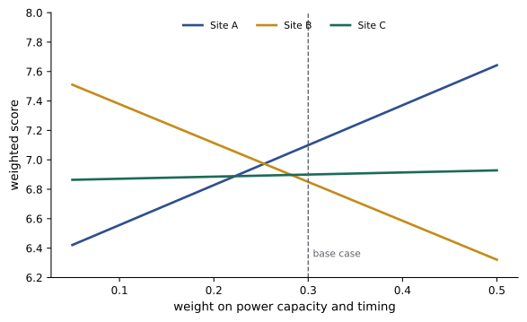
Site A ranks first in about two-thirds of the weight draws, so it is the leading candidate but not a certain one, and its lead depends on power being weighted at 25% or more. That points to the real question: how confident is the team in Site A's power advantage? If its energization date is firm, Site A is a sound choice; if it depends on a transmission upgrade not yet approved, its power score should be lower, and the ranking could flip. Sensitivity analysis thus directs due diligence to the facts that matter most.
Other techniques complement scoring:
- Total cost of ownership over the project life (land, construction, energy, taxes, water, network) for the finalists, converted to a present value, separates cost from qualitative factors.
- Scenario analysis tests the finalists against plausible futures: higher energy prices, a carbon price, a tightened water allocation, a delay in a transmission line.
- Portfolio thinking: experienced developers advance several sites in parallel, with land options and early utility applications, because some will fail for reasons no screening could predict. The cost of options and studies on sites that are dropped is the price of speed.
Worked problem
Value of a parallel site
A developer estimates that its preferred site has a 70% chance of obtaining power and zoning on schedule. A second site, independent of the first, has a 60% chance and would cost $2 million in options and studies to advance in parallel. A one-year delay would cost the business about $40 million. Is advancing the second site worthwhile?
Show solution
- Probability that both fail: \(0.30 \times 0.40 = 0.12\), compared with 0.30 for the preferred site alone.
- Reduction in delay probability: \(0.30 - 0.12 = 0.18\). Expected saving: \(0.18 \times 40 = \$7.2\) million.
Answer: An expected saving of about $7.2 million against a cost of $2 million: advancing the second site pays. Such calculations are rough, but they show why parallel paths are standard practice for large projects with critical deadlines.
Common mistakes
MistakeStarting the search before agreeing a written requirements brief.
InsteadDefine capacity, timing, latency, cost and fatal flaws first, so candidates can be screened consistently.
MistakeTreating every data center as latency-sensitive.
InsteadMatch location to the workload: AI training can go where power is; interconnection sites must be in network hubs.
MistakeRelying on one preferred site.
InsteadAdvance alternatives in parallel when deadlines are critical.
MistakeTreating weighted scores as precise.
InsteadTest sensitivity to weights and uncertain scores, and investigate the facts that drive the ranking.
MistakeKeeping a project secret until the council meeting.
InsteadPlan disclosure deliberately and engage the community before formal applications.
Summary and key terms
- Hyperscale, AI training, inference, colocation, enterprise and edge facilities have very different siting needs.
- Markets are tracked by inventory, absorption, vacancy and pipeline; power constraints increasingly govern supply.
- Fiber adds about 5 µs per kilometer one way; AI training campuses can be remote, while interconnection sites cannot.
- Searches proceed from a requirements brief through GIS-based screening to parcels, using utilities, agencies and brokers.
- Confidentiality protects negotiations but must give way to planned, credible public engagement.
- Sensitivity analysis, cost of ownership, scenarios and parallel sites make decisions robust.
- Hyperscale
- Very large cloud operators building campuses of hundreds of megawatts.
- Colocation
- Data center space, power and cooling leased to multiple customers.
- Absorption
- The amount of capacity leased in a market over a period.
- Route factor
- Fiber route length divided by straight-line distance.
- Requirements brief
- A document defining what a site must provide.
- Fatal flaw
- A condition that rules out a site regardless of other merits.
- GIS
- Geographic information system for combining spatial data layers.
- Site-ready program
- A utility or regional program certifying sites with known power, zoning and environmental status.
- Sensitivity analysis
- Testing how results change when inputs or weights vary.
- Parallel path
- Advancing alternative sites at the same time to reduce schedule risk.
Practice problems
Work each problem on paper first, then reveal the answer to check.
Which facility type is least sensitive to latency to users?
Show answer
AI training campuses.
One-way delay over 300 km of fiber?
Show answer
1.5 ms.
Round-trip propagation for a 200 km straight-line distance and route factor 1.5?
Show answer
3 ms.
A market absorbed 300 MW last year and has 450 MW unleased under construction. Years of supply?
Show answer
1.5 years.
Name three GIS layers used in screening.
Show answer
Transmission, fiber, flood zones (also gas, zoning, wetlands, parcels).
Give an example of a fatal flaw.
Show answer
No power before the deadline, or a site in a floodway.
Why do developers use code names and special-purpose companies?
Show answer
To avoid price escalation and premature opposition.
Two independent sites each have a 50% chance of success. Probability both fail?
Show answer
25%.
What does a site's first-place share of 60% in a weight sensitivity test indicate?
Show answer
It is favored but not robustly; the ranking depends on the weights.
What does a "site-ready" designation provide?
Show answer
Known power, zoning and environmental status, shortening due diligence.
Lesson quiz · 5 questions
Score 60% or more to complete this lesson.
Create a free account to save your progress, take quizzes and earn a certificate.