Pumps, piping and hydronic design

Water carries heat from the terminal units of Lesson 4 to the chillers and heat rejection of Lesson 5, and in liquid-cooled halls directly from the processors (Lesson 9). The hydronic system, its pumps, pipes, valves, controls and water treatment, decides how much energy that transport costs, whether every coil gets the flow it needs, and whether a single leak or failed pump can interrupt cooling. This lesson covers the heat-transport equation and temperature difference, pump and system curves, pipe sizing and pressure drop, pumping arrangements and their control, the problem of low temperature difference, glycol and water quality, and the redundancy features of a reliable loop.

Heat, flow and temperature difference

Water carries heat according to

For a given load, the flow needed is inversely proportional to the temperature difference between supply and return water. A 1 MW load needs 39.9 L/s at a 6 K difference, but only 23.9 L/s at 10 K. Because pumping power rises steeply with flow, the design temperature difference is one of the most important decisions in a cooling plant. Modern data center plants use differences of 8 K to 12 K or more, made possible by warm return air and the high return-water temperatures of liquid cooling.

Pump curves and system curves

A centrifugal pump adds pressure (expressed as head, in meters of water) that falls as flow rises; its pump curve, published by the manufacturer, shows head, efficiency and power against flow at a given speed. The piping system needs pressure to push water through it, rising roughly with the square of flow because friction losses do; this is the system curve. The pump operates where the two curves cross.

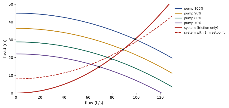
The affinity laws (the same as the fan laws of Lesson 3) relate pump performance to speed: flow is proportional to speed, head to speed squared, and power to speed cubed. Variable-speed drives exploit this.

import numpy as np

# Pump curve and system curve for a chilled-water loop
Q = np.linspace(0, 120, 1201)                 # L/s
H_pump_100 = 45.0 - 0.0015 * Q ** 2           # m of head at full speed
static = 0.0                                  # closed loop: no static lift
k = 25.0 / 90.0 ** 2                          # system: 25 m of friction at 90 L/s design flow

def operating_point(speed):
    H_pump = 45.0 * speed ** 2 - 0.0015 * Q ** 2   # affinity laws: head ~ speed^2
    H_sys = static + k * Q ** 2
    i = np.argmin(np.abs(H_pump - H_sys))
    return Q[i], H_sys[i]

eff = 0.78
for speed in (1.0, 0.9, 0.8, 0.7):
    q, h = operating_point(speed)
    power = 1000 * 9.81 * (q / 1000) * h / eff / 1000      # kW
    print(f"speed {speed:.0%}: flow {q:5.1f} L/s, head {h:4.1f} m, shaft power {power:5.1f} kW")

# The design flow needs a speed where the pump curve meets the system curve at 90 L/s
for speed in np.arange(0.70, 1.0, 0.001):
    if 45.0 * speed ** 2 - 0.0015 * 90 ** 2 >= k * 90 ** 2:
        print(f"speed for 90 L/s: {speed:.1%}")
        break

speed 100%: flow  99.1 L/s, head 30.3 m, shaft power  37.8 kW
speed 90%: flow  89.1 L/s, head 24.5 m, shaft power  27.5 kW
speed 80%: flow  79.2 L/s, head 19.4 m, shaft power  19.3 kW
speed 70%: flow  69.3 L/s, head 14.8 m, shaft power  12.9 kW
speed for 90 L/s: 90.9%

In a closed loop with only friction, flow is proportional to speed and power falls with the cube: at 70% speed the pump uses about a third of its full-speed power. Real systems are not quite so favorable, because controls hold a minimum differential pressure across the loop so that the farthest coils always have enough pressure to get their flow. The system curve then starts at that setpoint rather than at zero, and savings at low flow are smaller.

Pipes and pressure drop

Friction in pipes is calculated with the Darcy-Weisbach equation:

where \(f\) is the friction factor (about 0.015 to 0.025 for clean steel pipe in turbulent flow, from the Moody chart or the Colebrook equation), \(L\) the length, \(D\) the diameter and \(v\) the velocity. Fittings such as elbows, tees and valves add losses expressed as equivalent lengths or loss coefficients. Designers usually size pipes to keep velocities between about 1 and 3 m/s, balancing pipe cost against pumping energy, noise and erosion, or to a pressure-drop target such as 100 to 400 Pa/m.

Pumping arrangements

Primary-secondary

In a primary-secondary system, constant-speed primary pumps circulate a fixed flow through each chiller, and variable-speed secondary pumps distribute water to the load, with a short decoupling pipe (common pipe) between the circuits so their flows can differ. It was long the standard because older chillers needed constant evaporator flow. Its weakness is that when the load returns less flow than the chillers circulate, cold supply water short-circuits through the decoupler to the chiller inlet, lowering return temperature and plant efficiency.

Variable primary flow

Modern chillers tolerate varying evaporator flow within limits, so a single set of variable-speed pumps can serve both chillers and load. Variable primary flow saves pumps, space and energy, but needs careful control: a bypass valve to maintain each chiller's minimum flow, and slow rates of flow change so chillers can respond.

Control of the loop

Each coil has a two-way control valve that modulates flow to hold its air temperature. As valves close, loop pressure rises, and the pump drive slows to keep a differential pressure setpoint, measured near the far end of the loop (or reset by the control system to the lowest value that keeps the most-open valve nearly fully open). A valve controls well only if it has enough authority, meaning that its pressure drop when fully open is a substantial share, typically at least a quarter to a half, of the pressure drop across the circuit it controls. Pressure-independent control valves combine a regulator and a control valve so that flow depends only on the valve position.

Low temperature difference

Many chilled-water plants suffer from low ΔT syndrome: the return water comes back cooler than designed, so the same load needs more flow. The plant then runs more pumps and chillers than the load requires, each partly loaded, wasting energy and capacity.

# Why delta-T matters: flow and pumping power for a 5 MW chilled-water load
load_kw = 5000.0
ref_flow, ref_power = 199.0, 120.0        # L/s and kW of pumping at a 6 K design delta-T

for fluid, cp, rho, visc_factor in (("water", 4.18, 1000.0, 1.00), ("30% propylene glycol", 3.85, 1030.0, 1.25)):
    print(fluid)
    for dT in (6.0, 8.0, 10.0, 12.0):
        flow = load_kw / (cp * rho / 1000 * dT)               # L/s
        # in a fixed piping system pump power scales roughly with flow cubed;
        # higher viscosity raises friction, approximated by a factor on power
        power = ref_power * (flow / ref_flow) ** 3 * visc_factor
        print(f"  delta-T {dT:4.1f} K: flow {flow:6.1f} L/s, pumping about {power:6.1f} kW")

# Low delta-T syndrome: the plant designed for 10 K sees only 6 K
design, actual = 10.0, 6.0
print(f"at {actual:.0f} K instead of {design:.0f} K the plant must move {design / actual:.2f} times the water")

water
  delta-T  6.0 K: flow  199.4 L/s, pumping about  120.7 kW
  delta-T  8.0 K: flow  149.5 L/s, pumping about   50.9 kW
  delta-T 10.0 K: flow  119.6 L/s, pumping about   26.1 kW
  delta-T 12.0 K: flow   99.7 L/s, pumping about   15.1 kW
30% propylene glycol
  delta-T  6.0 K: flow  210.1 L/s, pumping about  176.6 kW
  delta-T  8.0 K: flow  157.6 L/s, pumping about   74.5 kW
  delta-T 10.0 K: flow  126.1 L/s, pumping about   38.2 kW
  delta-T 12.0 K: flow  105.1 L/s, pumping about   22.1 kW
at 6 K instead of 10 K the plant must move 1.67 times the water

Common causes, and their cures:

• Coils that are oversized, fouled or piped incorrectly, or three-way valves that bypass supply water into the return: replace three-way valves with two-way valves and maintain coils.
• Supply air setpoints that are too low, so coils open fully and pass water that is barely warmed: raise air setpoints within the ASHRAE range.
• Poor airflow management, so return air to the coils is cool: improve containment (Lesson 3).
• Decoupler flow in primary-secondary plants: convert to variable primary flow or control secondary flow to match primary.

Monitoring ΔT at each coil and at the plant, and trending it, is one of the most useful energy checks an operator can make.

Glycol, water quality and air

Loops exposed to freezing temperatures, such as dry coolers or economizer coils outdoors, are filled with a glycol solution. Glycol lowers the freezing point (30% propylene glycol protects to about −13 °C) but reduces specific heat and raises viscosity, so the same load needs more flow and more pumping energy, as the code above shows, and coil and heat exchanger capacities are derated. Many designs keep glycol only in the outdoor loop, separated from the indoor water by a plate heat exchanger.

Water quality matters for every loop, and especially for the secondary loops of liquid cooling, whose cold plates have channels a fraction of a millimeter wide:

• Treatment: corrosion inhibitors and biocides, with regular testing of pH, conductivity, inhibitor levels and bacteria.
• Filtration: strainers and side-stream filters remove particles; liquid-cooling loops typically filter to 25 to 50 µm or finer.
• Air removal: air separators and automatic vents remove air, which causes noise, corrosion and air locks; expansion tanks absorb thermal expansion and keep pressure above atmospheric everywhere so air cannot be drawn in.
• Materials: avoiding mixed metals in contact (for example copper and aluminum) that corrode galvanically.

Reliability in hydronic systems

Because a loss of water flow quickly stops cooling (Lesson 11 quantifies how quickly), loops are designed so that no single failure stops flow to the IT load:

• Pumps: N+1 or more, with automatic changeover, on separate power supplies, and with variable-speed drives that can be bypassed or replaced.
• Piping: looped (ring) headers or dual supply and return paths, so any section can be isolated and water reaches each unit from the other direction.
• Valves: isolation valves arranged so that maintenance or a leak isolates the smallest possible part of the system, and so that valves can be exercised regularly; valves that never move tend to seize.
• Leak detection: sensing cable under pipes and units, drip trays, and automatic isolation of leaking branches in liquid-cooled halls.
• Make-up water and storage: a supply to refill the loop, and in some plants chilled-water storage tanks that keep cooling running while chillers restart after a power interruption.