Calibration, linear regression and detection limits

A titration needs no calibration curve, because the result follows from stoichiometry. Most instrumental methods are different: an absorbance, a fluorescence intensity or a chromatographic peak area means nothing until it is compared with the response of standards. Calibration is the process of measuring standards of known concentration, fitting a mathematical relationship between signal and concentration, and using that relationship to convert the signal from an unknown into a concentration. Done well, calibration gives not only the concentration but its uncertainty, the range over which the method works, and the smallest amount it can detect. Done badly, it hides bias behind an impressive correlation coefficient.

Our running example is the determination of iron in water by spectrophotometry. Iron(II) forms an intensely red-orange complex with 1,10-phenanthroline, Fe(phen)₃²⁺, which absorbs strongly at 510 nm. Any iron(III) is first reduced to iron(II) with hydroxylamine, and the pH is held near 4 with an acetate buffer. By Beer's law, absorbance is proportional to concentration: A = εbc, where ε is the molar absorptivity (about 1.1 × 10⁴ L mol⁻¹ cm⁻¹ for this complex) and b is the path length.

Preparing standards

Calibration standards are prepared by accurate dilution of a stock solution, ideally one made from a primary standard or bought as a certified, traceable solution. Six standards spanning the expected range, including a blank (zero standard), are typical. They should be prepared in the same matrix as the samples as far as possible, with the same reagents added in the same order, so that any reagent absorbance and matrix effects are the same. Serial dilution saves stock but propagates any error from one step to the next; independent dilutions from the stock avoid that.

The method of least squares

If the response is linear, we want the straight line y = mx + b that best fits the n calibration points (xᵢ, yᵢ), with concentration x known accurately and signal y subject to random error. The method of least squares chooses m and b to minimize the sum of squared vertical deviations (residuals):

Setting ∂S/∂m = 0 and ∂S/∂b = 0 gives two linear equations (the normal equations). Their solution is

The line always passes through the centroid (x̄, ȳ). Squaring the residuals makes positive and negative deviations count equally and gives the most probable line when the errors in y are independent, normally distributed and of equal size (homoscedastic) at all concentrations.

How good is the fit?

The standard deviation about the regression, s_y (also called the standard error of the estimate), measures the scatter of points around the line:

The divisor n − 2 reflects the two parameters estimated from the data. The uncertainties of the slope and intercept follow:

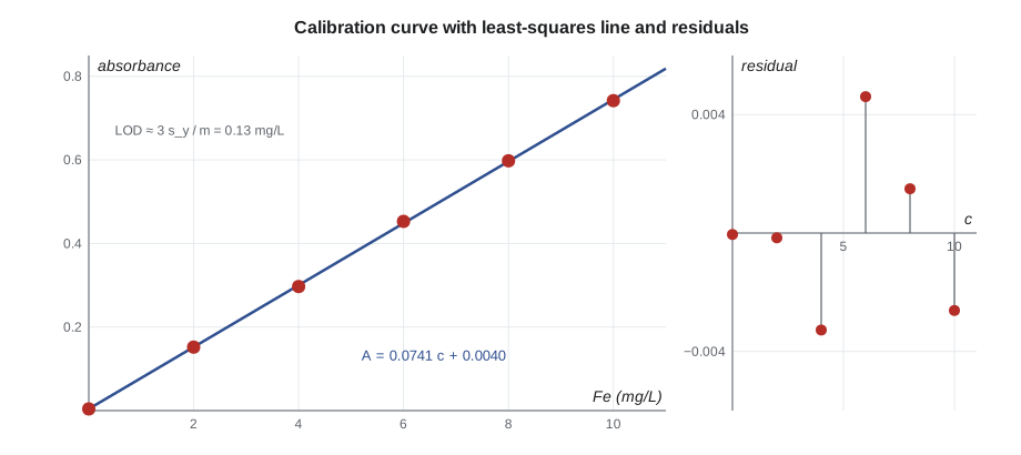
The correlation coefficient r and its square R² are often reported, but they are poor guides to the quality of a calibration. R² = 0.999 sounds excellent, yet it can hide a clear curve, a bias at low concentrations, or a single bad standard. Always look at the residual plot, which shows each residual against concentration. Random scatter about zero means the straight line is adequate; a systematic curve (residuals positive at the ends and negative in the middle, or the reverse) means the response is not linear; residuals that grow with concentration mean the errors are not uniform and weighted regression may be needed.

Finding the unknown and its uncertainty

An unknown giving signal y₀ (the mean of k replicate readings) has concentration x₀ = (y₀ − b)/m. Its standard uncertainty comes from the scatter of the unknown's readings, the uncertainty of the line, and where the unknown falls relative to the centroid:

The last term shows that uncertainty is smallest near the center of the calibration range and grows toward the ends. Unknowns should therefore fall near the middle of the standards, never outside them; extrapolation beyond the highest standard assumes a linearity that has not been demonstrated. Replicate readings of the unknown (larger k) reduce the first term, and more standards (larger n) reduce the second.

import math

x = [0.0, 2.0, 4.0, 6.0, 8.0, 10.0]          # Fe standards, mg/L
y = [0.004, 0.152, 0.297, 0.453, 0.598, 0.742] # absorbance at 510 nm
n = len(x)
xb, yb = sum(x) / n, sum(y) / n
Sxx = sum((xi - xb) ** 2 for xi in x)
Sxy = sum((xi - xb) * (yi - yb) for xi, yi in zip(x, y))
m = Sxy / Sxx
b = yb - m * xb
res = [yi - (m * xi + b) for xi, yi in zip(x, y)]
sy = math.sqrt(sum(r * r for r in res) / (n - 2))
sm = sy / math.sqrt(Sxx)
sb = sy * math.sqrt(sum(xi * xi for xi in x) / (n * Sxx))
r = Sxy / math.sqrt(Sxx * sum((yi - yb) ** 2 for yi in y))
print(f"slope m = {m:.5f} +/- {sm:.5f} per (mg/L)")
print(f"intercept b = {b:.5f} +/- {sb:.5f}")
print(f"s_y = {sy:.5f}; R^2 = {r * r:.5f}")
print("residuals:", ", ".join(f"{v:+.4f}" for v in res))

readings = [0.351, 0.347, 0.354]               # unknown, three readings
k = len(readings); y0 = sum(readings) / k
x0 = (y0 - b) / m
sx0 = sy / abs(m) * math.sqrt(1 / k + 1 / n + (y0 - yb) ** 2 / (m * m * Sxx))
t4 = 2.776                                      # Student t, 95 %, n - 2 = 4 df
print(f"unknown: x0 = {x0:.3f} mg/L, s = {sx0:.3f}, 95 % interval +/- {t4 * sx0:.2f} mg/L")
print(f"LOD = 3 s_y / m = {3 * sy / m:.2f} mg/L; LOQ = 10 s_y / m = {10 * sy / m:.2f} mg/L")

slope m = 0.07406 +/- 0.00038 per (mg/L)
intercept b = 0.00405 +/- 0.00232
s_y = 0.00321; R^2 = 0.99989
residuals: -0.0000, -0.0002, -0.0033, +0.0046, +0.0015, -0.0026
unknown: x0 = 4.680 mg/L, s = 0.031, 95 % interval +/- 0.09 mg/L
LOD = 3 s_y / m = 0.13 mg/L; LOQ = 10 s_y / m = 0.43 mg/L

Sensitivity, linear range and dynamic range

Sensitivity is the slope of the calibration curve, the change in signal per unit change in concentration. A steeper slope makes small differences in concentration easier to distinguish, but sensitivity alone does not determine how low a method can go: that depends also on the noise. The linear range extends from the lowest concentration that can be measured reliably to the concentration at which the response departs from linearity, often because of instrumental limitations (stray light in spectrophotometry, detector saturation) or chemical ones (incomplete complex formation, self-absorption). The dynamic range is the wider range over which there is any measurable response, linear or not.

Detection and quantitation limits

The detection limit (limit of detection, LOD) is the smallest concentration that gives a signal distinguishable from the blank with reasonable confidence. A common definition takes the signal that is three standard deviations of the blank above the mean blank:

where s_blank is the standard deviation of replicate blanks (at least seven are recommended) or of a very low standard. When blank replicates are unavailable, s_y from the calibration is sometimes used, as in the code above, though it usually overestimates the true detection limit at low concentration. The factor 3 gives roughly a 1 % chance that a blank alone would be reported as a detection (a false positive), but about a 50 % chance that a sample whose true concentration is exactly the LOD would be missed. The limit of quantitation (LOQ), the lowest concentration that can be measured with acceptable precision, is usually taken as 10 s_blank/m, about 3.3 times the LOD.

Regulatory agencies define detection limits in their own, more elaborate ways. The United States EPA's method detection limit procedure uses spiked samples and blanks analyzed over several days, and accredited laboratories in both Canada and the United States report results below their quantitation limit as less than the limit, rather than as a number that implies false precision. A result reported as below 0.5 µg/L lead does not mean there is no lead; it means the laboratory could not quantify it below that level.

Matrix effects and the method of standard additions

A calibration curve prepared in pure water assumes that the sample's matrix does not change the slope. Often it does. Dissolved organic matter may bind iron and slow complex formation; high salt concentrations change activity coefficients; in atomic spectroscopy, other elements change the efficiency of atomization. When the matrix changes the slope, results from an external calibration are biased.

The method of standard additions compensates by calibrating in the sample itself. Equal volumes of the unknown are placed in several flasks, increasing known amounts of a standard are added to all but one, and all are diluted to the same final volume. If the signal is proportional to concentration, a plot of signal against the concentration of added standard is a straight line whose x-intercept, extrapolated to negative values, gives the original concentration.

Here c_x′ is the unknown's concentration in the diluted flasks and c_s is the added standard's concentration in those flasks. The slope m is measured in the actual matrix, so a matrix effect that changes the slope is automatically included. Standard additions cannot correct for an additive interference (a background signal from the matrix that is present even without analyte), which must be removed by a proper blank. The extrapolation also amplifies uncertainty, so standard additions are more work and less precise than external calibration; they are used when the matrix is complex or variable.

cs = [0.0, 1.0, 2.0, 3.0]          # added Fe in the 50 mL flasks, mg/L
A = [0.165, 0.236, 0.310, 0.381]
n = len(cs); xb, yb = sum(cs) / n, sum(A) / n
Sxx = sum((x - xb) ** 2 for x in cs)
m = sum((x - xb) * (y - yb) for x, y in zip(cs, A)) / Sxx
b = yb - m * xb
sy = (sum((y - m * x - b) ** 2 for x, y in zip(cs, A)) / (n - 2)) ** 0.5
cx = b / m                          # concentration in the diluted flasks
# uncertainty of the extrapolated x-intercept
s_cx = sy / m * (1 / n + yb ** 2 / (m * m * Sxx)) ** 0.5
print(f"slope {m:.4f}, intercept {b:.4f}")
print(f"c in flasks = {cx:.3f} +/- {s_cx:.3f} mg/L")
print(f"well water = {cx * 50 / 10:.2f} +/- {s_cx * 50 / 10:.2f} mg/L (standard uncertainty)")

slope 0.0722, intercept 0.1647
c in flasks = 2.281 +/- 0.023 mg/L
well water = 11.41 +/- 0.12 mg/L (standard uncertainty)

Internal standards

An internal standard is a different substance, added in the same known amount to every standard and sample, whose signal responds to instrumental drift and sample-handling losses in the same way as the analyte's. Calibrating with the ratio of analyte signal to internal standard signal cancels these variations. Internal standards are essential in chromatography, where injection volumes vary, and in ICP-MS, where plasma conditions drift; isotopically labeled versions of the analyte make ideal internal standards in mass spectrometry. CHEM-311 develops these methods.

Good calibration practice

• Bracket the unknowns with standards; never extrapolate.
• Include a blank and at least five standards for a new method; check linearity with the residual plot.
• Run a check standard from an independent source to confirm that the calibration standards are correct.
• Recalibrate, or run a continuing calibration check, at intervals during a long run to catch drift.
• Match the matrix of standards to samples, or use standard additions or an internal standard when that is impossible.
• Report the uncertainty of the result, not just R².