
CHEM-211 · Lesson 4 of 12 · 25 min
Statistics of data: confidence intervals, t and F tests, outliers
Suppose your laboratory analyzes a certified reference material for iron and gets a mean of 19.70 mg/L from four replicates, while the certificate says 20.00 mg/L. Is the method biased, or is the difference just the random scatter you would expect from four measurements? Suppose two analysts measure the same water and get means of 131 and 127 mg/L hardness. Do they disagree? Suppose one result out of five looks suspiciously high. May you throw it out? Statistics answers such questions objectively, with a stated risk of being wrong. This lesson develops the tools analysts use most: the normal distribution, confidence intervals, Student's t tests, the F test and tests for outliers.
The normal distribution
If a measurement were repeated an enormous number of times, its random errors would usually follow a Gaussian or normal distribution, described by the population mean μ and the population standard deviation σ.
The curve is symmetric and bell-shaped. About 68.3 % of results lie within ±1σ of μ, 95.4 % within ±2σ, and 99.7 % within ±3σ; exactly 95 % lie within ±1.96σ. Random errors tend to be normally distributed because each result is the sum of many small independent effects, and the central limit theorem says that such sums approach a normal distribution whatever the distributions of the individual effects.
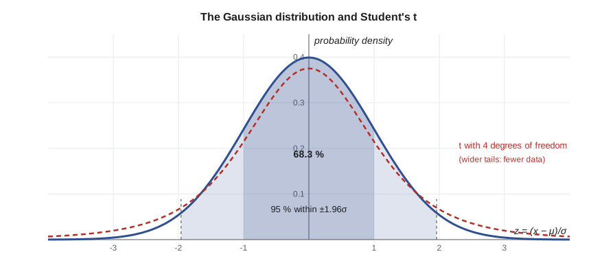
In practice we never know μ and σ; we estimate them by x̄ and s from a handful of results. With few results, s is itself uncertain, sometimes much smaller or larger than σ. William Sealy Gosset, a chemist at the Guinness brewery in Dublin who published in 1908 under the pen name Student, worked out the distribution that accounts for this extra uncertainty. Student's t distribution looks like the normal curve but with heavier tails; with more degrees of freedom it approaches the normal curve.
Confidence intervals
A confidence interval is a range around the mean that contains the true value with a stated probability, provided there is no systematic error:
Here t is Student's t for n − 1 degrees of freedom at the chosen confidence level, usually 95 %. With only a few data, t is large, so the interval is wide: for three replicates, t = 4.303 at 95 %, compared with 1.96 for infinitely many.
| Degrees of freedom | t (90 %) | t (95 %) | t (99 %) |
|---|---|---|---|
| 1 | 6.314 | 12.706 | 63.657 |
| 2 | 2.920 | 4.303 | 9.925 |
| 3 | 2.353 | 3.182 | 5.841 |
| 4 | 2.132 | 2.776 | 4.604 |
| 5 | 2.015 | 2.571 | 4.032 |
| 6 | 1.943 | 2.447 | 3.707 |
| 8 | 1.860 | 2.306 | 3.355 |
| 10 | 1.812 | 2.228 | 3.169 |
| 20 | 1.725 | 2.086 | 2.845 |
| ∞ | 1.645 | 1.960 | 2.576 |
Worked problem
A 95 % confidence interval
Four determinations of iron in a reference water give 19.62, 19.81, 19.58 and 19.79 mg/L. Find the 95 % confidence interval.
Show solution
- x̄ = 19.700 mg/L; s = 0.1169 mg/L; n = 4, 3 degrees of freedom, t = 3.182.
- ts/√n = 3.182 × 0.1169/2 = 0.186 mg/L.
Answer: μ = 19.70 ± 0.19 mg/L (95 % confidence). The interval 19.51 to 19.89 does not contain 20.00, so the next section tests whether this indicates bias.
A confidence interval has a precise meaning: if the whole experiment were repeated many times, 95 % of the intervals calculated this way would contain μ. It is not a statement that μ has a 95 % probability of lying in this particular interval, though for practical decisions the distinction rarely matters.
Hypothesis testing
Statistical tests compare a null hypothesis, which states that there is no real difference (the method is unbiased, the two means are equal), with an alternative. We compute a test statistic from the data and compare it with a critical value for the chosen significance level, usually α = 0.05. If the statistic exceeds the critical value, the difference is called statistically significant, and we reject the null hypothesis with a 5 % risk of being wrong (a type I error, a false alarm). Failing to reject does not prove the null hypothesis; the test may simply lack the power to detect a small real difference with few data (a type II error).
Statistical significance is not the same as practical importance. With enough data, a bias of 0.1 % can be statistically significant yet irrelevant to a decision about drinking water; with too few data, a bias of 5 % can go undetected. Always ask both whether a difference is real and whether it matters.
Comparing a mean with a known value
To test whether a mean differs from a certified or known value μ₀, compute
and compare it with the tabulated t for n − 1 degrees of freedom. This is equivalent to asking whether μ₀ lies outside the confidence interval.
Worked problem
Is the method biased?
For the iron data above (x̄ = 19.700, s = 0.1169, n = 4), is the difference from the certified value 20.00 mg/L significant at 95 %?
Show solution
- t_calc = |19.700 − 20.00| × √4 / 0.1169 = 0.300 × 2/0.1169 = 5.13.
- t_table (3 degrees of freedom, 95 %) = 3.182.
- 5.13 > 3.182, so the difference is significant (p ≈ 0.014).
Answer: The method reads low by about 1.5 %; look for a systematic error, such as incomplete reduction of iron or a degraded standard.
Comparing two means
When two sets of results are compared, for example two methods or two analysts, the test depends on whether the standard deviations are similar. If they are (checked with the F test below), pool them:
with n₁ + n₂ − 2 degrees of freedom. If the standard deviations differ significantly, Welch's version of the test uses each s separately and an adjusted number of degrees of freedom; the code below implements both.
A paired t test is used when each of several different samples is measured by both methods, for example ten water samples each analyzed by titration and by an instrument. The samples differ from one another, so the two sets cannot be pooled. Instead, compute the difference for each sample, d_i, and test whether the mean difference d̄ differs from zero: t = |d̄|√n/s_d with n − 1 degrees of freedom. Pairing removes the sample-to-sample variation and makes the test much more sensitive.
The F test for precision
To compare two standard deviations, compute F = s₁²/s₂², with the larger variance on top, and compare it with the critical F for (n₁ − 1, n₂ − 1) degrees of freedom. If F exceeds the critical value, the precisions differ significantly. The F test is used to decide whether a new method is more precise than an old one and whether the pooled t test is appropriate.
Outliers
An outlier is a result that seems inconsistent with the rest. The first step is always to look for a cause: a note in the notebook about a spill, a bubble in the burette, a misread balance. If there is a documented cause, the result is rejected for that reason. If not, a statistical test can help, but with few data no test can be very reliable, and discarding data to make results look better is a serious breach of scientific integrity.
The Grubbs test, recommended by ISO and ASTM, computes G = |questionable value − x̄|/s, with x̄ and s calculated from all the data including the suspect value. If G exceeds the critical value for n data (for a two-sided test at 95 % confidence, 1.154 for n = 3, 1.481 for 4, 1.715 for 5, 1.887 for 6, 2.020 for 7, 2.127 for 8, 2.290 for 10, 2.412 for 12), the value may be rejected. The older Dixon Q test uses the gap between the suspect value and its nearest neighbor divided by the range; it is still common in textbooks and teaching laboratories. Whatever the test, report how many values were rejected and why, and never apply an outlier test repeatedly to the same small data set.
Worked problem
A suspect result
Six chloride results (mg/L) are 30.2, 30.6, 30.4, 30.3, 31.9 and 30.5. Should 31.9 be retained?
Show solution
- x̄ = 30.65; s = 0.6285.
- G = |31.9 − 30.65|/0.6285 = 1.99.
- G_critical for n = 6 at 95 % (two-sided) is 1.887; 1.99 > 1.887.
Answer: The value 31.9 may be rejected as an outlier, provided the report says so; without it, x̄ = 30.40 mg/L, s = 0.16 mg/L.
import math

def betacf(a, b, x, itmax=300, eps=3e-14):
    """Continued fraction for the incomplete beta function (Numerical Recipes form)."""
    qab, qap, qam = a + b, a + 1, a - 1
    c, d = 1.0, 1 - qab * x / qap
    d = 1 / (d if abs(d) > 1e-300 else 1e-300); h = d
    for m in range(1, itmax + 1):
        m2 = 2 * m
        aa = m * (b - m) * x / ((qam + m2) * (a + m2))
        d = 1 + aa * d; c = 1 + aa / c; d = 1 / d; h *= d * c
        aa = -(a + m) * (qab + m) * x / ((a + m2) * (qap + m2))
        d = 1 + aa * d; c = 1 + aa / c; d = 1 / d; dl = d * c; h *= dl
        if abs(dl - 1) < eps: break
    return h

def ibeta(a, b, x):
    if x <= 0: return 0.0
    if x >= 1: return 1.0
    lb = math.lgamma(a + b) - math.lgamma(a) - math.lgamma(b) + a * math.log(x) + b * math.log(1 - x)
    if x < (a + 1) / (a + b + 2):
        return math.exp(lb) * betacf(a, b, x) / a
    return 1 - math.exp(lb) * betacf(b, a, 1 - x) / b

def t_two_tail_p(t, df):            # probability of |T| >= t
    return ibeta(df / 2, 0.5, df / (df + t * t))

def t_crit(df, conf=0.95):
    lo, hi = 0.0, 1000.0
    for _ in range(200):
        mid = (lo + hi) / 2
        if t_two_tail_p(mid, df) > 1 - conf: lo = mid
        else: hi = mid
    return mid

def f_upper_p(F, d1, d2):           # probability that F exceeds the value
    return ibeta(d2 / 2, d1 / 2, d2 / (d2 + d1 * F))

def mean_sd(x):
    m = sum(x) / len(x)
    return m, math.sqrt(sum((v - m) ** 2 for v in x) / (len(x) - 1))

for df in (2, 3, 4, 9):
    print(f"t(95 %, {df} df) = {t_crit(df):.3f}")

iron = [19.62, 19.81, 19.58, 19.79]
m, s = mean_sd(iron)
t = abs(m - 20.00) * math.sqrt(len(iron)) / s
print(f"iron: mean {m:.3f}, s {s:.4f}, t = {t:.2f}, p = {t_two_tail_p(t, len(iron) - 1):.4f}")

a = [131.2, 129.8, 130.5, 131.9, 130.6]     # analyst A, hardness mg/L
b = [127.4, 128.9, 126.6, 128.1, 127.8]     # analyst B
(ma, sa), (mb, sb) = mean_sd(a), mean_sd(b)
F = max(sa, sb) ** 2 / min(sa, sb) ** 2
print(f"F = {F:.2f}, p = {2 * f_upper_p(F, 4, 4):.3f} (two-sided)")
sp = math.sqrt((sa ** 2 * 4 + sb ** 2 * 4) / 8)
tp = abs(ma - mb) / sp * math.sqrt(25 / 10)
print(f"pooled t = {tp:.2f} with 8 df, critical {t_crit(8):.3f}, p = {t_two_tail_p(tp, 8):.5f}")
se2 = sa ** 2 / 5 + sb ** 2 / 5
dfw = se2 ** 2 / ((sa ** 2 / 5) ** 2 / 4 + (sb ** 2 / 5) ** 2 / 4)
tw = abs(ma - mb) / math.sqrt(se2)
print(f"Welch t = {tw:.2f} with {dfw:.1f} df, p = {t_two_tail_p(tw, dfw):.5f}")

def grubbs_crit(n, alpha=0.05):
    tc = t_crit(n - 2, 1 - alpha / n)
    return (n - 1) / math.sqrt(n) * math.sqrt(tc * tc / (n - 2 + tc * tc))
cl = [30.2, 30.6, 30.4, 30.3, 31.9, 30.5]
m, s = mean_sd(cl)
G = max(abs(v - m) for v in cl) / s
print(f"Grubbs G = {G:.3f}, critical (n = 6) = {grubbs_crit(6):.3f}")t(95 %, 2 df) = 4.303 t(95 %, 3 df) = 3.182 t(95 %, 4 df) = 2.776 t(95 %, 9 df) = 2.262 iron: mean 19.700, s 0.1169, t = 5.13, p = 0.0143 F = 1.16, p = 0.891 (two-sided) pooled t = 5.85 with 8 df, critical 2.306, p = 0.00038 Welch t = 5.85 with 8.0 df, p = 0.00039 Grubbs G = 1.989, critical (n = 6) = 1.887
The code computes the t and F distributions from the regularized incomplete beta function, so it does not need printed tables. It reports p values, the probability of a result at least this extreme if the null hypothesis were true. A p value below 0.05 corresponds to significance at the 95 % level. The two analysts differ by about 3 mg/L with a p value far below 0.01, a real difference. Since both cannot be right, the laboratory should look for a cause, for example different interpretations of the endpoint color change, which is a classic source of analyst bias in hardness titrations.
How many replicates?
Statistics also helps plan experiments. To estimate a mean to within ±E with 95 % confidence, n must be large enough that ts/√n ≤ E. Because t itself depends on n, solve by trial: with s = 0.12 mg/L and E = 0.10 mg/L, n = 8 gives 2.365 × 0.12/√8 = 0.100. Analysts typically run triplicates for routine work and more when a result is near a regulatory limit, where the decision depends on whether the confidence interval includes the limit.
Common mistakes
MistakeUse z = 1.96 with three replicates.
InsteadWith few data use Student's t for n − 1 degrees of freedom; for n = 3 it is 4.303.
MistakeA non-significant test proves there is no bias.
InsteadIt means the data cannot detect a difference of that size; more data might.
MistakePool the results of different samples measured by two methods.
InsteadUse a paired t test on the differences.
MistakeReject any result that looks high.
InsteadLook for a documented cause first, then apply one recognized test, once, and report it.
MistakeCompute s for the Grubbs test without the suspect value.
InsteadGrubbs uses the mean and s of all the data, including the suspect value.
MistakeStatistically significant means important.
InsteadA tiny bias can be significant with many data; judge whether it matters for the decision.
Summary and key terms
- Random errors usually follow a normal distribution; 95 % of values lie within ±1.96σ.
- With small samples use Student's t: μ = x̄ ± ts/√n.
- Compare a mean with a known value using t = |x̄ − μ₀|√n/s.
- Compare two means with a pooled t test (similar precision), Welch's test (different precision) or a paired t test (different samples measured both ways).
- Compare precisions with F = s₁²/s₂².
- Outliers may be rejected with the Grubbs test only after looking for a cause; always report rejections.
- Statistical significance does not by itself mean practical importance.
- Normal distribution
- The symmetric bell-shaped distribution of random errors, defined by μ and σ.
- Student's t
- A factor larger than z that widens confidence intervals for small samples.
- Confidence interval
- A range around the mean expected to contain the true value with a stated probability.
- Null hypothesis
- The assumption, tested statistically, that there is no real difference.
- Significance level
- The accepted risk of wrongly rejecting the null hypothesis, usually 0.05.
- Paired t test
- A t test on the differences between two measurements of the same samples.
- F test
- A comparison of two variances.
- Grubbs test
- A test for a single outlier based on its distance from the mean in units of s.
Practice problems
Work each problem on paper first, then reveal the answer to check.
Five results have x̄ = 7.36 and s = 0.08. Give the 95 % confidence interval.
Show answer
t (4 df) = 2.776; 2.776 × 0.08/√5 = 0.099; 7.36 ± 0.10.
A reference material certified at 50.0 gives x̄ = 49.2, s = 0.6, n = 6. Is there bias at 95 %?
Show answer
t = 0.8 × √6/0.6 = 3.27 > 2.571; yes.
Method A: s = 0.35 (n = 6); method B: s = 0.15 (n = 6). Critical F (5, 5, 95 % two-sided) is 7.15. Do the precisions differ?
Show answer
F = 0.1225/0.0225 = 5.44 < 7.15; no significant difference.
Two means, 25.3 and 24.8, each from 4 results with s_pooled = 0.30. Is the difference significant at 95 %?
Show answer
t = 0.5/0.30 × √(16/8) = 2.36 < 2.447 (6 df); not significant.
Results 10.2, 10.4, 10.3, 11.1: may 11.1 be rejected by Grubbs at 95 % (critical 1.481)?
Show answer
x̄ = 10.50, s = 0.408; G = 1.47 < 1.481, so it must be retained, however odd it looks.
How does the 95 % interval change when going from 3 to 12 replicates, if s is unchanged?
Show answer
From 4.303s/√3 = 2.48s to 2.201s/√12 = 0.64s, nearly four times narrower.
Lesson quiz · 5 questions
Score 60% or more to complete this lesson.
Create a free account to save your progress, take quizzes and earn a certificate.