
CHEM-211 · Lesson 3 of 12 · 23 min
Errors, uncertainty and propagation
No measurement is exact. A balance reading fluctuates in its last digit, a burette reading depends on how the meniscus is judged, a standard may be slightly impure, and a reaction may not go quite to completion. An analytical result is therefore incomplete without an estimate of its uncertainty: a range within which the true value is believed to lie with stated confidence. A blood alcohol result of 0.081 g per 100 mL means one thing if the uncertainty is ±0.001 and something very different if it is ±0.005, when the legal limit is 0.080. This lesson classifies the errors that affect measurements, shows how to describe them with numbers, and develops the rules for propagating uncertainty through a calculation.
Kinds of error
Error is the difference between a measured value and the true value. The true value is never known exactly, but it can be approached through careful work and reference materials. Errors fall into three classes.
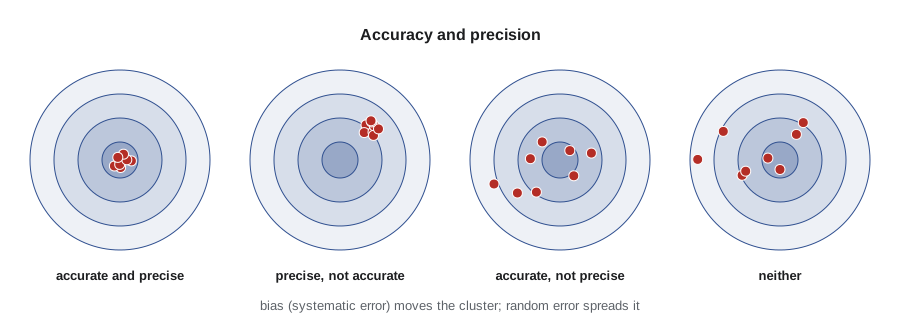
Systematic errors (determinate errors) have a definite cause and, in principle, can be found and corrected. They make results consistently high or consistently low. Their sources include the method (an indicator that changes slightly after the equivalence point, a precipitate that is slightly soluble, an interference), the instrument (a burette whose true volumes differ from its markings, a pH meter calibrated with an old buffer), and the person (always reading a meniscus from slightly above, consistently overshooting an endpoint). Systematic error is also called bias.
Random errors (indeterminate errors) arise from many small, uncontrollable fluctuations: electrical noise, tiny variations in drainage of a pipette, judgment of the last digit on a scale, air currents around the balance. They scatter results on both sides of the mean, are equally likely to be positive or negative, and can be reduced by averaging replicates but never eliminated.
Gross errors (blunders) are mistakes: a spilled sample, a misread digit, a transposed number in a notebook, the wrong reagent. They produce outliers that are far from the other results. They should be prevented by careful work, caught by quality control, and documented when they occur; statistical tests for outliers (lesson 4) help decide whether a suspect value can be discarded.
Accuracy and precision
Accuracy is closeness to the true value; it is limited by systematic error. Precision is closeness of replicate results to one another; it is limited by random error. The figure shows the four combinations as shots at a target. Good precision is necessary for good accuracy but not sufficient: a tight cluster can be far from the center if there is a bias, and a scattered set can have a mean that happens to be near the center.
Absolute error is the measured value minus the accepted value, with its sign and units. Relative error is the absolute error divided by the accepted value, usually expressed in % or in parts per thousand (ppt, ‰). If a reference material certified at 20.00 mg/L iron is measured as 19.70 mg/L, the absolute error is −0.30 mg/L and the relative error is −1.5 %, or −15 ‰.
Detecting systematic errors
Because systematic errors do not show up as scatter, they must be found deliberately. Analysts use four strategies:
- Analyze a certified reference material (CRM) whose composition is known and traceable, and compare the result with the certified value (lesson 4 shows how to test the difference statistically).
- Compare with an independent method based on a different principle; agreement between, say, a titration and an instrumental method makes a common bias unlikely.
- Analyze blanks to detect contamination and reagent contributions, and spiked samples (samples with a known amount of analyte added) to measure recovery.
- Vary the sample size. A constant error, such as a fixed loss of 0.3 mg of precipitate, matters more for small samples; a proportional error, such as an interference present at a fixed fraction of the analyte, has the same relative effect at all sizes. Comparing results for different sample sizes distinguishes them.
Describing random error
For a set of n replicate results x₁, x₂, …, xₙ, the mean is the best estimate of the central value, and the sample standard deviation s describes the spread.
The divisor n − 1, the number of degrees of freedom, appears because the deviations are measured from the sample mean, which was itself computed from the data; one piece of information has been used up. The relative standard deviation RSD = s/x̄, often given in % and then called the coefficient of variation, allows precision to be compared across different concentrations. The variance is s². The standard deviation of the mean, s/√n, shows how much more reliable a mean of several results is than a single result: four replicates halve the uncertainty of the mean, but halving it again needs sixteen.
Worked problem
Mean and standard deviation
Five titrations of a vinegar sample give acetic acid concentrations of 0.8342, 0.8361, 0.8337, 0.8355 and 0.8349 M. Find the mean, s, RSD and standard deviation of the mean.
Show solution
- Mean = 4.1744/5 = 0.83488 M.
- Deviations (×10⁻⁴): −6.8, +12.2, −11.8, +6.2, +0.2; squares sum to 3.584 × 10⁻⁶.
- s = √(3.584 × 10⁻⁶/4) = 9.47 × 10⁻⁴ M; RSD = 0.113 %.
- Standard deviation of the mean = 9.47 × 10⁻⁴/√5 = 4.2 × 10⁻⁴ M.
Answer: 0.8349 M, s = 0.0009 M (RSD 0.11 %), standard deviation of the mean 0.0004 M.
Propagation of uncertainty
Most results are calculated from several measured quantities, each with its own uncertainty. If the uncertainties are random and independent, they partly cancel, so they do not simply add. The general rule follows from a first-order Taylor expansion. For a result y = f(x₁, x₂, …) with standard uncertainties u(x₁), u(x₂), …,
Why squares? A small change δx₁ in x₁ changes y by (∂f/∂x₁)δx₁. The variance of a sum of independent random changes is the sum of their variances, because the cross terms average to zero when the changes are uncorrelated. Applying this to common functions gives the familiar rules.
| Calculation | Rule for the uncertainty in y |
|---|---|
| y = a + b or y = a − b | u(y)² = u(a)² + u(b)² (absolute uncertainties add in quadrature) |
| y = ab or y = a/b | (u(y)/y)² = (u(a)/a)² + (u(b)/b)² (relative uncertainties add in quadrature) |
| y = aⁿ | u(y)/y = |n| u(a)/a |
| y = log₁₀ a | u(y) = 0.4343 u(a)/a |
| y = 10ᵃ | u(y)/y = 2.303 u(a) |
| y = ka (k exact) | u(y) = k u(a) |
The log rule explains why pH is quoted to two decimal places: an uncertainty of ±0.01 in pH corresponds to a relative uncertainty of 2.303 × 0.01 = 2.3 % in [H⁺]. A pH meter calibrated to ±0.02 pH units therefore cannot give [H⁺] better than about 5 %.
Worked problem
Uncertainty in a concentration
A 0.5132 ± 0.00014 g sample of KHP (204.22 g/mol) requires 25.07 ± 0.03 mL of NaOH. Find the concentration of NaOH and its uncertainty, ignoring the tiny uncertainty in the molar mass and KHP purity.
Show solution
- c = m/(M V) = 0.5132/(204.22 × 0.02507) = 0.10024 M.
- Relative uncertainties: mass 0.00014/0.5132 = 0.027 %; volume 0.03/25.07 = 0.120 %.
- Combined relative uncertainty = √(0.027² + 0.120²) = 0.123 %.
- u(c) = 0.00123 × 0.10024 = 0.00012 M.
Answer: c = 0.1002 ± 0.0001 M; the burette volume dominates the uncertainty.
The example shows a general lesson: the largest relative uncertainty dominates, because squares of small numbers are tiny. Improving the balance would do almost nothing; using a larger titrant volume or a better burette would help. An uncertainty budget, a table of every contribution and its share of the total, shows where effort pays off.
import random, statistics

# Standardization of NaOH with KHP: c = m * P / (M * V)
m, um = 0.5132, 0.00014      # g
P, uP = 0.99995, 0.00010     # purity (mass fraction) from the certificate
M, uM = 204.221, 0.004       # g/mol
V, uV = 25.07e-3, 0.03e-3    # L

c = m * P / (M * V)
budget = {'mass': um / m, 'purity': uP / P, 'molar mass': uM / M, 'volume': uV / V}
rel = sum(r ** 2 for r in budget.values()) ** 0.5
print(f"c = {c:.5f} M, u(c) = {c * rel:.5f} M ({rel * 100:.3f} % relative)")
for k, r in budget.items():
    print(f"  {k:10s} {r * 100:.4f} %   share of variance {r ** 2 / rel ** 2 * 100:5.1f} %")

# Monte Carlo check: sample every input from its distribution
rnd = random.Random(211)
sims = [rnd.gauss(m, um) * rnd.gauss(P, uP) / (rnd.gauss(M, uM) * rnd.gauss(V, uV)) for _ in range(100000)]
print(f"Monte Carlo: mean {statistics.fmean(sims):.5f} M, sd {statistics.stdev(sims):.5f} M")c = 0.10023 M, u(c) = 0.00012 M (0.123 % relative) mass 0.0273 % share of variance 4.9 % purity 0.0100 % share of variance 0.7 % molar mass 0.0020 % share of variance 0.0 % volume 0.1197 % share of variance 94.4 % Monte Carlo: mean 0.10023 M, sd 0.00012 M
The Monte Carlo method in the code is a powerful general alternative to the propagation formulas: draw many random values for each input from its distribution, compute the result for each set, and take the standard deviation of the results. It handles nonlinear functions and correlated inputs that the first-order formula treats poorly, and it is the basis of a supplement to the international Guide to the Expression of Uncertainty in Measurement (GUM).
Standard and expanded uncertainty
The GUM, first published in 1993 and maintained by the Joint Committee for Guides in Metrology, is the international framework for evaluating and reporting uncertainty. It distinguishes Type A evaluations, made statistically from repeated measurements (a standard deviation of the mean), from Type B evaluations, made by other means (a manufacturer's tolerance, a certificate, a handbook value). Both are expressed as standard uncertainties and combined by the propagation rule to give the combined standard uncertainty u_c.
A tolerance quoted as ±a, with no other information, is usually treated as a rectangular distribution, in which any value in the interval is equally likely; its standard uncertainty is a/√3. A Class A 25 mL pipette with tolerance ±0.03 mL therefore contributes a standard uncertainty of 0.03/√3 = 0.017 mL. A triangular distribution, in which values near the center are more likely, gives a/√6.
For reporting, the combined standard uncertainty is multiplied by a coverage factor k, usually 2, to give the expanded uncertainty U = k u_c. For a roughly normal distribution, an interval of ±2u_c contains the true value with about 95 % confidence. The report should say what was done, for example: iron 19.70 ± 0.24 mg/L, where the uncertainty is an expanded uncertainty with coverage factor k = 2.
Propagation in spectrophotometry
Propagation also explains why instruments have a best working range. In absorption spectrophotometry the concentration is proportional to the absorbance A = −log T, where T is the fraction of light transmitted. If the error in reading T is roughly constant, the relative error in concentration is (0.4343 u_T)/(T A), which is large when the solution absorbs almost nothing (T near 1, A near 0) and when it absorbs almost everything (T near 0). Setting the derivative to zero shows a minimum at A = 0.4343.
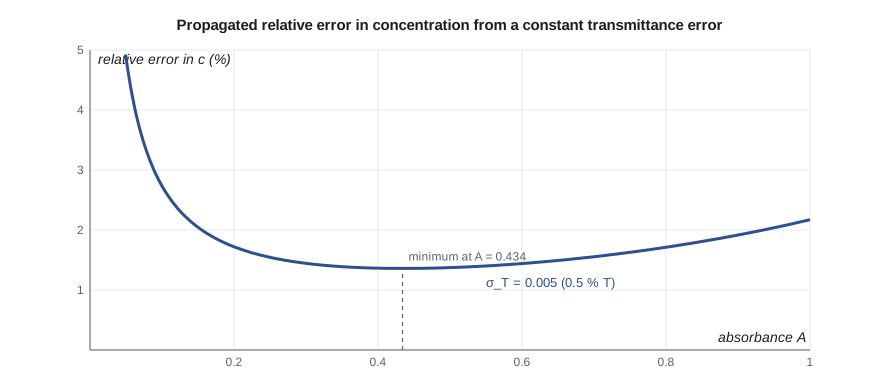
For this reason calibration standards and samples are usually diluted to give absorbances between about 0.2 and 0.8. Modern instruments whose noise is not constant in T have somewhat different optimum ranges, but the principle is general: work where the propagated uncertainty is smallest.
Common mistakes
MistakeAdd absolute uncertainties for a product.
InsteadFor products and quotients, combine relative uncertainties in quadrature.
MistakeAdd uncertainties linearly.
InsteadIndependent random uncertainties combine as the square root of the sum of squares.
MistakeGood precision proves good accuracy.
InsteadA biased method can be very precise; check against a reference material or independent method.
MistakeUse n instead of n − 1 for a sample standard deviation.
InsteadThe n − 1 divisor accounts for the degree of freedom used by the sample mean.
MistakeTreat a tolerance ±a as a standard uncertainty.
InsteadUnless stated otherwise, divide by √3 (rectangular distribution).
MistakeReport a result without saying what the uncertainty means.
InsteadState whether it is a standard deviation, a confidence interval or an expanded uncertainty with its coverage factor.
Summary and key terms
- Systematic errors cause bias and affect accuracy; random errors cause scatter and affect precision; gross errors are blunders.
- Systematic errors are found with certified reference materials, independent methods, blanks, spikes and varied sample sizes.
- The sample standard deviation uses n − 1; the standard deviation of the mean falls as 1/√n.
- Independent uncertainties combine in quadrature: absolute for sums and differences, relative for products and quotients.
- The largest relative uncertainty dominates; an uncertainty budget shows where to improve.
- The GUM combines Type A and Type B standard uncertainties and reports an expanded uncertainty U = k u_c, usually with k = 2.
- Propagation explains optimum working ranges, such as absorbances of about 0.2 to 0.8.
- Systematic error
- A reproducible error with a definite cause that biases results in one direction.
- Random error
- Unpredictable variation that scatters results about the mean.
- Accuracy
- Closeness of a result to the true value.
- Precision
- Closeness of replicate results to one another.
- Relative standard deviation
- The standard deviation divided by the mean.
- Uncertainty budget
- A table of the contributions to the combined uncertainty of a result.
- Combined standard uncertainty
- The standard uncertainty of a result obtained by propagating the standard uncertainties of its inputs.
- Expanded uncertainty
- The combined standard uncertainty multiplied by a coverage factor, usually 2.
Practice problems
Work each problem on paper first, then reveal the answer to check.
A CRM certified at 1.250 % N gives 1.231 % N. Find the absolute and relative error.
Show answer
−0.019 % N; −1.5 % relative (−15 ‰).
Find the uncertainty in 43.27 ± 0.03 − 12.85 ± 0.03 mL.
Show answer
30.42 ± √(0.03² + 0.03²) = 30.42 ± 0.04 mL.
Find c and its uncertainty for c = n/V with n = 2.502 ± 0.004 mmol and V = 50.00 ± 0.05 mL.
Show answer
c = 0.05004 M; relative u = √(0.160² + 0.100²) % = 0.189 %; u(c) = 0.00009 M.
A pH is 4.37 ± 0.02. Find [H⁺] and its uncertainty.
Show answer
[H⁺] = 4.27 × 10⁻⁵ M; relative u = 2.303 × 0.02 = 4.6 %; u = 0.20 × 10⁻⁵ M.
What standard uncertainty does a 100 mL flask with tolerance ±0.08 mL contribute?
Show answer
0.08/√3 = 0.046 mL.
How many replicates are needed to cut the standard deviation of the mean to one-third of s?
Show answer
√n = 3, so n = 9.
Lesson quiz · 5 questions
Score 60% or more to complete this lesson.
Create a free account to save your progress, take quizzes and earn a certificate.