
APT-210 · Lesson 5 of 12 · 28 min
Inventory turns and carrying cost
▶ Video coming soon A video version of this lesson is on the way.
Every month, Walter Bisset, the general manager, met with each department head to go over the numbers. Rolf brought Talia to the parts department's meeting in October so she could see how the department was judged. Walter skipped past the sales figures and stopped at one line. "Turns are 6.0," he said. "The Linmore group target is 6.5. What's holding us back?" Rolf had the answer ready: about 38,000 dollars of parts that had not sold in a year, and a handful of parts stocked far too deep. Talia realised that a single number was telling the general manager a great deal about the warehouse she worked in every day.
Lesson 1 introduced inventory turns and carrying cost. This lesson looks at both more closely: how turns are calculated for the whole department and for single parts, what makes them rise or fall, what carrying cost is made of, and how the order quantity affects the balance between ordering costs and carrying costs.
Calculating turns
Inventory turns measure how many times a year the department sells and replaces its average inventory:
Two details matter. First, both numbers must be at cost, the price the department paid, not the selling price. Using sales at selling price would make turns look higher than they are. Second, the inventory figure should be an average over the year, not the value on one day, because inventory rises and falls with orders and seasons. Many departments average the month-end values for the last twelve months.
Worked problem
An average inventory from month-end values
The month-end inventory at cost for the last four months was 612,000, 655,000, 648,000 and 630,000 dollars. What is the average for those months?
Show solution
- Total:
- \[612{,}000 + 655{,}000 + 648{,}000 + 630{,}000 = 2{,}545{,}000\]
- Average:
- \[2{,}545{,}000 \div 4 = 636{,}250\]
Answer: The average is 636,250 dollars. A twelve-month average works the same way with twelve values. Using a single month-end value can make turns look better or worse than they really were.
For Linmore Tessaro over the past year, the cost of parts sold was 3,840,000 dollars and the average inventory at cost was 640,000 dollars, giving 6.0 turns. Turns can also be calculated for a shorter period and converted to a yearly rate: if the department sold 320,000 dollars of parts at cost in one month with 640,000 dollars of inventory, it turned 0.5 times that month, which is 6.0 a year.
Turns for a single part
Turns can also be calculated part by part. This is where the department's overall figure comes from: some parts turn many times a year, others hardly at all, and the department's turns are the combined result.
Worked problem
Turns for a fast-moving part
A brake pad set costs the department 22 dollars. In the past year it sold 48 sets, and the department kept an average of 4 sets on hand. How many times did it turn?
Show solution
- Cost of the sets sold:
- \[48 \times 22 = 1{,}056\]
- Average inventory at cost:
- \[4 \times 22 = 88\]
- Turns:
- \[1{,}056 \div 88 = 12.0\]
Answer: The pad set turned 12 times a year, twice the department average. For a single part, turns are simply units sold divided by the average units on hand, because the cost cancels out: 48 ÷ 4 = 12.
| Part type | Typical turns pattern |
|---|---|
| Maintenance parts: filters, wipers, pads | High; sell every week |
| Common repair parts: sensors, belts, bulbs | Moderate |
| Collision and body parts | Low if stocked; usually special-ordered |
| Slow movers kept for service | Low; one or two sales a year |
| Non-moving parts | Zero; drag the department's turns down |
A department's overall turns can be raised in two ways: by selling more from the same inventory, or by holding less inventory for the same sales. The second is usually where the improvement comes from. Getting rid of non-moving stock (lesson 6) and trimming parts stocked far deeper than their demand needs both lower the average inventory without losing sales.
What good turns look like
There is no single right number for turns. Manufacturers and dealer groups often publish targets for their dealers, and figures around 5 to 8 turns a year are common goals for dealership parts departments that carry a full range of parts for their make. A store that sells mostly fast-moving maintenance parts can turn faster; a store that must stock many slow parts for older models or heavy equipment will turn slower. In this course, the Linmore group target of 6.5 turns is a sample value.
Turns should always be read alongside the fill rate. A department that raises its turns from 6.0 to 7.5 by cutting stock across the board may see its fill rate fall, lose customers and use more emergency orders. A department that raises turns by clearing parts that never sell, while keeping fast movers in stock, improves both. Rolf told Walter that he could reach 6.5 turns by spring without lowering the fill rate, by returning or clearing the non-moving parts and correcting a list of parts stocked too deep.
What carrying cost is made of
Carrying cost, or holding cost, is the cost of keeping inventory on hand for a year. It is usually expressed as a share of the inventory's value. Its main parts are:
- The cost of money: the interest on money borrowed to buy the stock, or the return the dealership gives up by having its cash on the shelf instead of elsewhere.
- Storage and handling: the building space, shelving, heating, lighting and the staff time spent moving, counting and caring for stock.
- Obsolescence: parts that stop selling and lose value because models change, parts are superseded or technology moves on.
- Shrink and damage: parts lost, stolen, broken or damaged in storage (lesson 8).
- Insurance and taxes: insurance on the stock and, in some places, property or inventory taxes.
Worked problem
Breaking down the carrying cost
Rolf estimated these sample rates for a year: cost of money 7 in 100, storage and handling 6 in 100, obsolescence 8 in 100, shrink and damage 2 in 100, insurance and taxes 2 in 100. What is the total rate, and what does it cost to carry 640,000 dollars of inventory?
Show solution
- Total rate:
- \[7 + 6 + 8 + 2 + 2 = 25\ \text{in}\ 100\]
- Cost of money:
- \[640{,}000 \times 0.07 = 44{,}800\]
- Storage and handling:
- \[640{,}000 \times 0.06 = 38{,}400\]
- Obsolescence:
- \[640{,}000 \times 0.08 = 51{,}200\]
- Shrink, insurance and taxes:
- \[640{,}000 \times 0.04 = 25{,}600\]
- Total:
- \[44{,}800 + 38{,}400 + 51{,}200 + 25{,}600 = 160{,}000\]
Answer: The total sample rate is 25 in 100, or 160,000 dollars a year. Obsolescence is the largest part, which is why lesson 6's work on non-moving stock matters so much.
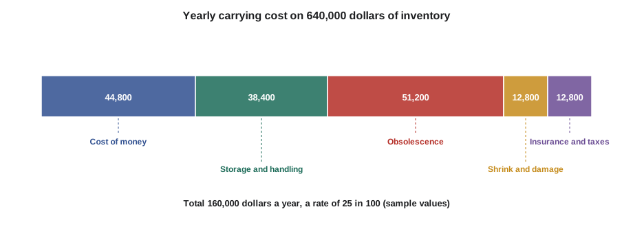
The rates vary from one business to another. Interest rates change, building costs differ, and a department with careful stock control loses less to obsolescence. Rolf's figures were estimates, but even rough estimates help: they show that a part sitting unsold on the shelf for a year has cost the dealership about a quarter of its value, on top of whatever it will fetch when it is finally sold.
Order quantity: ordering cost against carrying cost
How many of a part to buy at a time involves another balance. Each order has a cost: the time to review and place it, receive it, check it and put it away, and any freight. Ordering less often in larger quantities lowers these ordering costs but raises the average inventory, and so the carrying cost. Ordering more often in smaller quantities does the reverse.
The economic order quantity (EOQ) is a classic formula for the order quantity that keeps the total of ordering and carrying costs as low as possible:
Here D is the yearly demand in units, S is the cost of placing and receiving one order, and H is the yearly cost of carrying one unit, which is the unit cost times the carrying cost rate.
Worked problem
An economic order quantity
A filter sells 1,100 a year and costs the department 6.80 dollars. Rolf estimates the cost of handling one order of it at 12 dollars, and uses a carrying rate of 25 in 100. What is the EOQ?
Show solution
- Carrying cost per unit:
- \[H = 6.80 \times 0.25 = 1.70\]
- EOQ:
- \[\sqrt{\dfrac{2 \times 1{,}100 \times 12}{1.70}} = \sqrt{15{,}529} \approx 124.6\]
- Round to the package quantity:
- 125, if the filter comes in boxes of 25
- Orders a year:
- \[1{,}100 \div 125 = 8.8\]
- Yearly ordering cost:
- \[8.8 \times 12 = 105.60\]
- Yearly carrying cost:
- \[(125 \div 2) \times 1.70 = 106.25\]
Answer: The EOQ is about 125 filters. At that quantity, the yearly ordering cost (about 106 dollars) and carrying cost (about 106 dollars) are almost equal, which is where the total is lowest. All costs here are sample values.
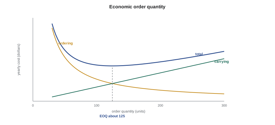
In practice, dealers rarely use the EOQ formula part by part. Most parts come in on a weekly stock order, so the ordering cost of adding one more line is small, and the order quantity is set by min/max rules instead (lesson 3). The EOQ idea still matters for parts bought separately from other suppliers, for very high-volume items such as oil and fluids, and for understanding why buying a year's supply to get a small discount often costs more than it saves.
Quantity discounts and forward buying
Suppliers sometimes offer a discount for buying large quantities, or a special price for a limited time. Forward buying, buying more than normal now to save on price, can make sense, but only when the saving is larger than the extra carrying cost and the risk that the parts will not sell.
Worked problem
Is a quantity discount worth it?
A supplier offers 4 in 100 off a battery if the department buys a six-month supply instead of a one-month supply. The carrying rate is 25 in 100 a year. Roughly, is the discount worth it?
Show solution
- Average extra time on the shelf:
- about 2.5 months longer for the extra batteries, on average
- Extra carrying cost for that time:
- \[0.25 \times 2.5 \div 12 \approx 0.052, \text{ or about 5 in 100}\]
- Compare:
- a 4 in 100 discount against about 5 in 100 extra carrying cost
Answer: The discount is not quite worth it at this carrying rate, and the risk of batteries aging on the shelf makes it worse. A larger discount, or a shorter buy, could change the answer. The figures are sample values.
Rolf's general rule was cautious: forward buy only parts that sell steadily, will not change or age quickly, and are not likely to be superseded. Batteries, which lose charge and have a shelf life, and parts for models about to change, are poor candidates.
Turns by group
A department's overall turns hide large differences between groups of parts. Fast-moving maintenance parts such as filters, wiper blades and brake pads may turn 10 or more times a year. Slow but necessary parts, such as body panels for older models or major engine parts, may turn once a year or less. The overall figure is an average of all these groups, weighted by how much money each holds.
Looking at turns by group, by ABC class or by source shows where the money is working and where it is not. At Linmore Tessaro, Rolf's report showed that A parts turned about 11 times a year, B parts about 5 and C parts under 2. The C parts held less than a quarter of the inventory value, but they were where most of the non-moving stock was found. That told him where to look first when Walter asked for higher turns: not at the A parts, which were working hard already, but at the slow C parts and the settings that had stocked them.
Raising turns by cutting fast-moving parts is a common mistake. It lowers the fill rate on the parts customers ask for most, and it saves little carrying cost because fast parts do not sit on the shelf for long anyway.
The lesson for parts technicians is that turns are a tool for finding problems, not a score to chase. A department with honest, well-set stocking levels and a good fill rate will usually find that its turns follow.
Common mistakes
MistakeCalculating turns from sales at selling price.
InsteadUse the cost of parts sold and the inventory at cost.
MistakeUsing one month-end inventory value.
InsteadUse an average over the year.
MistakeRaising turns by cutting all stock.
InsteadClear non-moving and overstocked parts and keep fast movers in stock.
MistakeTreating carrying cost as just interest.
InsteadInclude storage, obsolescence, shrink and insurance.
MistakeForward buying whenever there is a discount.
InsteadCompare the discount with the extra carrying cost and the risk.
Summary and key terms
- Turns = cost of parts sold ÷ average inventory at cost; for a single part, units sold ÷ average units on hand.
- Read turns alongside the fill rate; raise turns by clearing stock that does not sell.
- Carrying cost includes the cost of money, storage and handling, obsolescence, shrink and insurance; 25 in 100 is this course's sample rate.
- EOQ balances ordering cost against carrying cost; it is lowest where the two are about equal.
- Most dealer parts are ordered by min/max on the stock order, but the EOQ idea explains why big buys can cost more than they save.
- Forward buy only steady, stable parts, and only when the saving beats the carrying cost.
- Average inventory
- The average inventory value over a period, often from month-end values.
- At cost
- Valued at the price the department paid, not the selling price.
- Holding cost
- Another name for carrying cost.
- Obsolescence
- Loss of value when parts stop selling because models or parts change.
- Economic order quantity
- The order quantity that minimizes the total of ordering and carrying costs.
- Forward buying
- Buying more than normal now to save on price.
Practice problems
Work each problem on paper first, then reveal the answer to check.
Cost of parts sold is 1,800,000 dollars; average inventory at cost is 360,000 dollars. What are the turns?
Show answer
1,800,000 ÷ 360,000 = 5.0.
A part sold 30 units in a year with an average of 5 on hand. How many turns?
Show answer
30 ÷ 5 = 6.
What is the yearly carrying cost of 50,000 dollars of stock at 25 in 100?
Show answer
12,500 dollars.
D = 800, S = 10 dollars, H = 2 dollars. What is the EOQ?
Show answer
√(2 × 800 × 10 ÷ 2) = √8,000 ≈ 89.
Name two ways to raise turns without hurting the fill rate.
Show answer
Clear non-moving stock and trim parts stocked far deeper than their demand.
Lesson quiz · 5 questions
Score 60% or more to complete this lesson.
Create a free account to save your progress, take quizzes and earn a certificate.