
AI-350 · Lesson 9 of 12 · 31 min
Video and 3D vision
The world is three-dimensional and changes over time, but a single image is a flat snapshot. Many of the most demanding vision applications, such as self-driving vehicles, robots, augmented reality headsets, drones, sports analytics and security systems, must understand motion and recover the 3D structure of their surroundings. This lesson covers how motion is estimated between frames, how objects are tracked, how actions in video are recognized, how depth is recovered from stereo cameras, motion and active sensors, how 3D scenes are reconstructed and represented, and the special demands of safety-critical systems that act on what they see.
Video as data
A video is a sequence of frames, typically 24 to 60 per second, so it adds a time dimension to the image tensor: \(T \times H \times W \times 3\). Consecutive frames are highly redundant, which video codecs exploit by storing occasional full frames and, between them, only motion and differences. Vision systems must decide how many frames to process and at what resolution, because processing every frame of high-resolution video with a large model is expensive. Common strategies sample a few frames per second, process a low-resolution stream continuously and switch to high resolution when something interesting appears, or reuse computation between similar frames.
Worked problem
Video compute budget
A detector needs 20 GFLOPs per 1080p frame. A city deploys it on 500 cameras at 15 frames per second. What sustained compute is needed, and how many accelerators delivering an effective 50 TFLOP/s each?
Show solution
- Per camera: \(20 \times 15 = 300\) GFLOP/s.
- Total: \(500 \times 300 = 150{,}000\) GFLOP/s \(= 150\) TFLOP/s.
- Accelerators: \(150/50 = 3\).
Answer: 150 TFLOP/s, about three accelerators at the assumed effective rate, before allowing for peaks, redundancy and tracking. Halving the frame rate or resolution, or processing only frames with motion, cuts the cost proportionally.
Optical flow
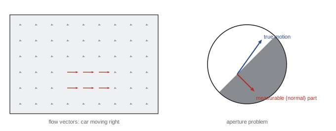
Optical flow is the apparent motion of each pixel between two frames, a 2D vector field \((u, v)\). It is used for video stabilization, motion segmentation, frame interpolation, action recognition and as an input to tracking. The classical approach assumes brightness constancy: a point keeps its brightness as it moves, so for small motions:
where \(I_x\), \(I_y\) are spatial gradients and \(I_t\) the temporal change. This is one equation in two unknowns per pixel. The Lucas-Kanade method assumes the flow is constant in a small window and solves the resulting over-determined system by least squares. The solution is reliable only if the window contains gradients in two directions; along a straight edge, motion parallel to the edge is invisible, the aperture problem.
import numpy as np

# Lucas-Kanade optical flow for one small window, on a smooth synthetic image that moves by (u, v)
yy, xx = np.mgrid[0:40, 0:40].astype(float)
def scene(dx, dy):
    X, Y = xx - dx, yy - dy
    return np.sin(X / 4.0) + np.cos(Y / 5.0) + 0.5 * np.sin((X + Y) / 6.0)

u_true, v_true = 0.6, -0.4
I0, I1 = scene(0, 0), scene(u_true, v_true)
Ix = np.gradient(I0, axis=1); Iy = np.gradient(I0, axis=0); It = I1 - I0
win = (slice(15, 26), slice(15, 26))       # 11 x 11 window
A = np.stack([Ix[win].ravel(), Iy[win].ravel()], axis=1)
b = -It[win].ravel()
u, v = np.linalg.lstsq(A, b, rcond=None)[0]
print(f"estimated flow u = {u:.3f}, v = {v:.3f}  (true {u_true}, {v_true})")
eig = np.linalg.eigvalsh(A.T @ A)
print(f"eigenvalues of the structure matrix: {eig[0]:.1f}, {eig[1]:.1f}  (both large: well-conditioned window)")

# a window on a pattern that varies only along x (an edge): the aperture problem
edge = np.sin(xx / 4.0)
Ixe = np.gradient(edge, axis=1)[win].ravel(); Iye = np.gradient(edge, axis=0)[win].ravel()
eig_e = np.linalg.eigvalsh(np.stack([Ixe, Iye], 1).T @ np.stack([Ixe, Iye], 1))
print(f"edge-only window eigenvalues: {eig_e[0]:.1f}, {eig_e[1]:.1f} (one is zero: vertical motion is invisible)")estimated flow u = 0.604, v = -0.446 (true 0.6, -0.4) eigenvalues of the structure matrix: 2.1, 6.4 (both large: well-conditioned window) edge-only window eigenvalues: 0.0, 3.3 (one is zero: vertical motion is invisible)
In a textured window, the estimated flow (0.60, −0.45) is close to the true motion (0.6, −0.4); the small error comes from approximating the image linearly over a shift of half a pixel. The 2 × 2 structure matrix has two substantial eigenvalues, so both components are determined. On a pattern varying only horizontally, one eigenvalue is zero: vertical motion cannot be measured, however good the algorithm. Modern learned methods such as RAFT (2020) estimate dense flow with deep networks, handling large motions, occlusions and textureless regions far better, using context from the whole image.
Tracking
Multi-object tracking follows detected objects across frames, assigning each a consistent identity. The common tracking-by-detection approach runs a detector on each frame, predicts where each existing track should be using a motion model (often a Kalman filter assuming roughly constant velocity), and associates new detections with tracks by solving an assignment problem on a cost combining IoU, distance and appearance similarity (an embedding of each object's appearance, as in DeepSORT). Unmatched detections start new tracks; tracks without detections for several frames are ended. Difficulties include occlusion, crowded scenes where people cross, identity switches, and objects leaving and re-entering the view. Tracking is evaluated by metrics such as MOTA and HOTA, which combine detection errors with identity errors.
Worked problem
Constant-velocity prediction
A tracked car's box center was at (400, 300) pixels two frames ago and (412, 302) in the last frame. Predict its center in the next frame. A detection appears at (425, 303); another at (480, 310). Which should be associated, using distance?
Show solution
- Velocity: (12, 2) pixels per frame. Prediction: (424, 304).
- Distances: to (425, 303): \(\sqrt{1 + 1} = 1.4\) px; to (480, 310): \(\sqrt{56^2 + 6^2} = 56.3\) px.
Answer: The detection at (425, 303) matches the prediction within 1.4 pixels and is associated with the track; the other is a different object and starts or continues another track. A Kalman filter adds uncertainty estimates so that the gate for association widens when the track is uncertain.
Action and video recognition
Recognizing actions (a person falling, a goal being scored, a hand reaching for an item) requires modeling motion over time. Approaches have progressed from two-stream networks (one CNN on frames, another on optical flow), to 3D CNNs (I3D, SlowFast) that convolve over space and time, to video transformers (TimeSformer, ViViT, VideoMAE) that attend over space-time patches, often with factorized attention (spatial then temporal) to control cost. Large video-language models now describe and answer questions about videos, but long videos remain challenging because of the number of tokens involved.
Depth from stereo
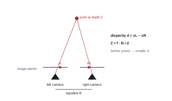
With two cameras a known distance apart (the baseline \(B\)), a point appears at slightly different horizontal positions in the two images. After rectification, which aligns the images so matching points lie on the same row, the horizontal shift is the disparity \(d\), and depth follows from similar triangles:
where \(f\) is the focal length in pixels. Depth is inversely proportional to disparity, so depth resolution degrades quickly with distance: the depth error from a fixed disparity error grows with the square of depth.
import numpy as np

# rectified stereo pair: depth Z = f * B / d
f_px, B = 1000.0, 0.12                 # focal length (pixels) and baseline (m)
for d in (60.0, 20.0, 6.0, 2.0):
    Z = f_px * B / d
    dZ = Z**2 / (f_px * B) * 0.25        # depth error for a 0.25 px disparity error
    print(f"disparity {d:5.1f} px -> depth {Z:6.2f} m  (+/- {dZ:.2f} m for 0.25 px error)")

# block matching on a synthetic scanline: find the shift that best aligns a patch
rng = np.random.default_rng(1)
left = rng.random(200)
true_d = 7
right = np.roll(left, -true_d) + rng.normal(0, 0.02, 200)
x, w = 100, 5
patch = left[x - w:x + w + 1]
costs = [np.sum((patch - right[x - dd - w:x - dd + w + 1]) ** 2) for dd in range(0, 20)]
print("sum of squared differences by disparity 0-19:", np.round(costs, 2))
print("best disparity:", int(np.argmin(costs)), " true:", true_d)disparity 60.0 px -> depth 2.00 m (+/- 0.01 m for 0.25 px error) disparity 20.0 px -> depth 6.00 m (+/- 0.07 m for 0.25 px error) disparity 6.0 px -> depth 20.00 m (+/- 0.83 m for 0.25 px error) disparity 2.0 px -> depth 60.00 m (+/- 7.50 m for 0.25 px error) sum of squared differences by disparity 0-19: [2.19 1.56 1.3 1.07 1.66 0.56 1.17 0. 1.16 0.68 1. 1.27 0.89 2.13 1.15 1.87 1.55 2.02 1.81 2.12] best disparity: 7 true: 7
With a 1000-pixel focal length and a 12 cm baseline, a quarter-pixel disparity error means about 1 cm of depth error at 2 m but 7.5 m at 60 m. This is why stereo systems for driving use wider baselines and higher resolutions for distant objects, and why lidar or radar complements cameras at range. Finding disparities requires matching each pixel to its partner in the other image; the block-matching example finds the correct 7-pixel disparity as the shift with the lowest sum of squared differences. Matching fails in textureless regions, repeated patterns and occlusions, which learned stereo networks handle better.
Structure from motion, SLAM and depth sensors
A single moving camera can also recover 3D structure: features matched across frames constrain both the camera's motion and the 3D positions of the points, which are estimated together by bundle adjustment, a large nonlinear least-squares optimization. Structure from motion (SfM) reconstructs scenes from collections of photos, used for mapping, heritage documentation and creating 3D models. Simultaneous localization and mapping (SLAM) does this in real time, letting robots, drones and AR headsets track their position while building a map, often fusing camera data with inertial measurements (visual-inertial odometry). Monocular systems recover structure only up to an unknown scale, which another sensor or known object size must fix.
Active depth sensors measure depth directly. Time-of-flight cameras and lidar emit light and time its return; lidar scanners on vehicles measure millions of points per second at ranges of 200 m or more. Structured light projects a known pattern and measures its distortion, as in some face-unlock systems. Radar measures range and velocity robustly in rain and fog but at low resolution. Learned monocular depth estimation predicts depth from a single image using cues such as perspective, object sizes and shading; large models trained on diverse data now produce impressively consistent relative depth, though absolute scale remains uncertain.
| Method | Strengths | Limitations |
|---|---|---|
| Stereo cameras | Passive, dense, inexpensive | Fails on textureless surfaces; error grows with depth squared |
| Lidar | Accurate range to 200 m+, works in darkness | Cost, sparse at range, degraded by heavy rain, fog, snow |
| Radar | Velocity, works in bad weather | Low resolution |
| Time-of-flight and structured light | Dense depth at short range | Sunlight interference, limited range |
| Monocular learned depth | Single camera, dense | Scale ambiguity; errors on unusual scenes |
Representing 3D scenes
Reconstructed or sensed 3D data are represented as point clouds (sets of 3D points, processed by networks such as PointNet that are invariant to point order), voxel grids (3D pixels), meshes (vertices and triangles) or implicit functions. Neural radiance fields (NeRF, 2020) represent a scene as a neural network mapping a 3D position and viewing direction to color and density, trained from posed photographs, producing photorealistic novel views. 3D Gaussian splatting (2023) represents scenes as millions of small colored 3D Gaussians that can be rendered in real time, quickly becoming the preferred method for capturing real places for visualization, games, real estate and digital twins, including of data centers and industrial facilities.
Worked problem
Point cloud density
A lidar measures 1.2 million points per second over a 360° × 30° field of view, rotating 10 times per second. Roughly how many points fall on a pedestrian 0.5 m wide and 1.7 m tall at 50 m, assuming points are spread evenly?
Show solution
- Points per rotation: 120,000 over \(360° \times 30° = 10{,}800\) square degrees, about 11.1 points per square degree.
- Pedestrian angular size at 50 m: width \(0.5/50 = 0.01\) rad \(= 0.57°\); height \(1.7/50 = 0.034\) rad \(= 1.95°\); area \(1.12\) square degrees.
- Points: \(11.1 \times 1.12 \approx 12\).
Answer: Only about a dozen points per scan, enough to detect that something is there but not to recognize it reliably. Combining lidar with high-resolution cameras (sensor fusion) is how most automated driving systems handle distant objects.
Safety-critical vision
When vision systems control vehicles, robots or medical decisions, errors can injure people. Such systems require more than high average accuracy: they need performance guarantees across rare situations (unusual vehicles, emergency workers, children, extreme weather), redundancy among sensors with different failure modes, monitoring that detects when inputs fall outside the conditions the system was designed for, conservative behavior under uncertainty, extensive simulation and on-road or clinical testing, and safety cases that argue systematically why risk is acceptable. Standards such as ISO 26262 (functional safety) and ISO 21448 (safety of the intended functionality, which addresses performance limitations of sensors and algorithms) guide automotive development.
In the US, the National Highway Traffic Safety Administration sets federal vehicle safety standards and, through its Standing General Order, requires manufacturers and operators to report crashes involving automated driving systems and advanced driver assistance; it has opened investigations and recalls based on such reports. States regulate testing and deployment on public roads, with California, Arizona and Texas among those hosting commercial robotaxi services under varying permit regimes. Medical imaging AI is regulated by the FDA as a medical device, with hundreds of AI-enabled devices authorized, most in radiology.
Lesson 10 develops the geometry behind stereo and structure from motion, and Lesson 12 covers the deployment of vision systems.
Common mistakes
MistakeProcessing every frame of every camera at full resolution.
InsteadMatch frame rate and resolution to the task; trigger heavier processing on events.
MistakeTrusting optical flow along edges or in textureless regions.
InsteadCheck the structure matrix or use learned methods that use wider context.
MistakeExpecting stereo depth to stay accurate at long range.
InsteadDepth error grows with Z²; widen the baseline or add lidar or radar.
MistakeAssuming monocular reconstruction gives true scale.
InsteadFix scale with another sensor or known dimensions.
MistakeValidating safety-critical vision on average accuracy alone.
InsteadTest rare scenarios, add redundancy and out-of-distribution monitoring, and build a safety case.
Summary and key terms
- Video adds a time dimension; frame rate and resolution drive compute cost.
- Optical flow estimates pixel motion; Lucas-Kanade solves Ixu + Iyv + It = 0 by least squares in windows.
- The aperture problem prevents measuring motion along an edge.
- Tracking-by-detection predicts tracks with motion models and associates detections by IoU, distance and appearance.
- Action recognition uses two-stream networks, 3D CNNs and video transformers.
- Stereo depth Z = fB/d; depth error grows with the square of depth.
- Structure from motion and SLAM recover 3D structure and camera motion; lidar, radar and ToF sense depth actively.
- Point clouds, meshes, NeRF and Gaussian splatting represent 3D scenes; safety-critical systems need redundancy and safety cases.
- Optical flow
- The apparent per-pixel motion between frames.
- Brightness constancy
- The assumption that a moving point keeps its intensity.
- Aperture problem
- The impossibility of measuring motion along an edge from local data.
- Kalman filter
- A recursive estimator combining motion predictions with measurements.
- Multi-object tracking
- Following many objects across frames with consistent identities.
- Disparity
- The horizontal shift of a point between rectified stereo images.
- Baseline
- The distance between stereo cameras.
- Structure from motion
- Recovering 3D structure and camera poses from images.
- SLAM
- Simultaneous localization and mapping.
- Lidar
- A sensor measuring distance by timing reflected laser pulses.
- Neural radiance field
- A neural representation of a scene's color and density for view synthesis.
- Gaussian splatting
- Representing a scene as many 3D Gaussians for real-time rendering.
Practice problems
Work each problem on paper first, then reveal the answer to check.
A 4K video (3840 × 2160) at 30 fps: pixels per second?
Show answer
About 249 million.
Write the optical flow constraint equation.
Show answer
Ix u + Iy v + It = 0.
Why does Lucas-Kanade fail on a straight edge?
Show answer
Gradients point in one direction only, so motion along the edge is unconstrained (one eigenvalue zero).
Box centers at (100, 50) then (106, 48). Constant-velocity prediction for the next frame?
Show answer
(112, 46).
f = 800 px, B = 0.3 m, d = 12 px. Depth?
Show answer
20 m.
Same system: depth error for a 0.5 px disparity error at 20 m?
Show answer
400/240 × 0.5 = 0.83 m.
How does depth error scale when distance doubles?
Show answer
It quadruples.
What does bundle adjustment optimize?
Show answer
3D point positions and camera poses together, minimizing reprojection error.
Name two strengths each of lidar and radar.
Show answer
Lidar: accurate long range, works in darkness. Radar: measures velocity, robust in bad weather.
What does ISO 21448 address?
Show answer
Safety of the intended functionality: hazards from performance limitations of sensors and algorithms.
Lesson quiz · 5 questions
Score 60% or more to complete this lesson.
Create a free account to save your progress, take quizzes and earn a certificate.