Inside modern detectors and dense prediction

Lesson 5 introduced the detection and segmentation tasks, IoU, non-maximum suppression, average precision and the main families of detectors. This lesson opens up the detectors to see how they are trained and why recent designs work better: how candidate predictions are assigned to ground-truth objects, why focal loss solves the imbalance between objects and background, how box regression losses are defined, how DETR-style detectors use bipartite matching to avoid duplicate removal, and how dense prediction extends to panoptic segmentation, human pose estimation and promptable segmentation. It ends with practical strategies for small objects, high-resolution images and real-time deployment.

Dense prediction and assignment

One-stage detectors such as RetinaNet, FCOS and the YOLO family make a prediction at every location of several feature maps in a feature pyramid. A typical 640 × 640 input produces feature maps with strides of 8, 16 and 32 pixels, giving 80 × 80, 40 × 40 and 20 × 20 grids, or 8,400 locations, each predicting class scores and a box, and anchor-based designs multiply this by several anchor shapes per location. During training, each ground-truth object must be assigned to one or more of these predictions, which become positives; all others are negatives (background).

• Anchor-based assignment (Faster R-CNN, RetinaNet, early YOLO) compares preset anchor boxes of several sizes and aspect ratios with each object and marks anchors with IoU above a threshold (for example 0.5) as positives and below another (0.4) as negatives. Anchor shapes must suit the data, for example tall, thin anchors for pedestrians.
• Anchor-free assignment (FCOS, CenterNet, recent YOLO versions) treats locations inside or near the center of an object as positives and predicts distances to the box edges directly, removing the need to design anchors.
• Dynamic assignment (ATSS, SimOTA, task-aligned assignment) chooses positives adaptively for each object based on how well each prediction currently scores, balancing classification and localization quality.

Assignment is one of the details that most affect detector accuracy, and much of the progress in YOLO versions since 2020 has come from better assignment, augmentation and training recipes rather than new backbones.

Focal loss and the imbalance problem

With thousands of locations per image and only a handful of objects, the vast majority of training examples are easy background, such as sky and road, which the model quickly learns to classify correctly with high confidence. Each easy example contributes only a small cross-entropy loss, but there are so many that together they dominate the gradient and swamp the useful signal from objects and hard background. Focal loss (RetinaNet, 2017) multiplies the cross-entropy by a modulating factor that shrinks the loss for well-classified examples:

where \(p_t\) is the predicted probability of the true class and \(\gamma\) (typically 2) controls how strongly easy examples are down-weighted; \(\alpha_t\) balances positives and negatives.

import numpy as np

# Why focal loss: a dense detector sees ~100,000 candidate locations per image, almost all easy background
n_easy, n_hard_bg, n_obj = 100000, 1000, 20
p_easy, p_hard, p_obj = 0.01, 0.40, 0.60          # predicted object probability for each group

def ce(p, y):
    return -np.log(p if y == 1 else 1 - p)

def focal(p, y, gamma=2.0, alpha=0.25):
    pt = p if y == 1 else 1 - p
    a = alpha if y == 1 else 1 - alpha
    return -a * (1 - pt) ** gamma * np.log(pt)

for name, f in (("cross-entropy", ce), ("focal loss (gamma 2)", focal)):
    L_easy = n_easy * f(p_easy, 0)
    L_hard = n_hard_bg * f(p_hard, 0)
    L_obj = n_obj * f(p_obj, 1)
    tot = L_easy + L_hard + L_obj
    print(f"{name:22s}: easy background {L_easy / tot:6.1%}, hard background {L_hard / tot:6.1%}, objects {L_obj / tot:6.1%} of the total loss")
# Box overlap measures: IoU and generalized IoU (GIoU) for boxes that do not overlap
def iou_giou(a, b):
    ix = max(0, min(a[2], b[2]) - max(a[0], b[0])); iy = max(0, min(a[3], b[3]) - max(a[1], b[1]))
    inter = ix * iy
    area = lambda r: (r[2] - r[0]) * (r[3] - r[1])
    union = area(a) + area(b) - inter
    cx = (max(a[2], b[2]) - min(a[0], b[0])) * (max(a[3], b[3]) - min(a[1], b[1]))
    return inter / union, inter / union - (cx - union) / cx
gt = (10, 10, 50, 50)
for pred in ((12, 14, 52, 50), (60, 10, 100, 50), (150, 10, 190, 50)):
    iou, giou = iou_giou(gt, pred)
    print(f"prediction {pred}: IoU {iou:.2f}, GIoU {giou:+.2f}")

cross-entropy         : easy background  65.9%, hard background  33.5%, objects   0.7% of the total loss
focal loss (gamma 2)  : easy background   0.1%, hard background  99.2%, objects   0.7% of the total loss
prediction (12, 14, 52, 50): IoU 0.82, GIoU +0.81
prediction (60, 10, 100, 50): IoU 0.00, GIoU -0.11
prediction (150, 10, 190, 50): IoU 0.00, GIoU -0.56

Under cross-entropy, 100,000 easy background locations account for two thirds of the loss even though each is classified with 99% confidence. Focal loss cuts their share to 0.1%, so training concentrates on the hard examples near the decision boundary. In practice, the loss is normalized by the number of positive locations so that objects receive adequate weight.

Box regression losses

Detectors predict box coordinates as offsets from an anchor or a location. Early detectors used L1 or smooth L1 losses on the four coordinates, but these treat each coordinate independently and do not directly optimize the overlap measure used in evaluation. IoU-based losses, \(1 - \text{IoU}\), optimize overlap directly but give zero gradient when boxes do not overlap. Generalized IoU (GIoU) subtracts the fraction of the smallest enclosing box not covered by the union, so it remains informative for non-overlapping boxes and pulls them together; Distance-IoU and Complete-IoU add terms for the distance between centers and the aspect ratio, speeding convergence. As the code above shows, two non-overlapping predictions both have IoU 0, but GIoU correctly scores the nearer one higher.

Set prediction with DETR

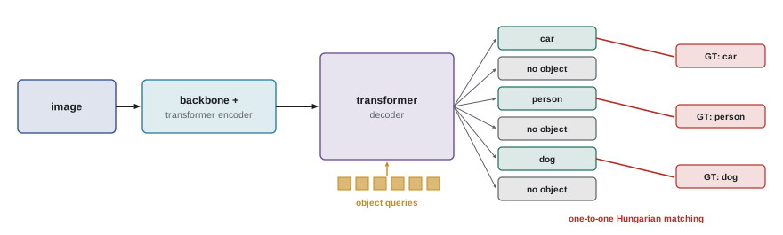
Dense detectors produce many overlapping predictions for each object and rely on non-maximum suppression (Lesson 5) to remove duplicates, a hand-designed step with a threshold that can suppress genuinely overlapping objects in crowds. DETR (detection transformer, 2020) reformulates detection as direct set prediction. A CNN or transformer backbone produces image features; a transformer decoder takes a fixed set of learned object queries, typically 100 to 300, each of which attends to the image features and outputs one class (including "no object") and one box. During training, the predictions are matched one to one with the ground-truth objects by the Hungarian algorithm, which finds the assignment that minimizes the total matching cost of classification and box errors. Matched queries are trained toward their objects; unmatched queries are trained to predict "no object".

import numpy as np
from scipy.optimize import linear_sum_assignment

# DETR-style set prediction: match 6 predicted object queries to 3 ground-truth objects with the Hungarian algorithm
gt = [("car", (20, 30, 120, 90)), ("person", (150, 20, 180, 100)), ("dog", (60, 70, 100, 110))]
preds = [  # (probabilities for car, person, dog, no-object), box
    ((0.70, 0.05, 0.05, 0.20), (25, 32, 118, 92)),
    ((0.10, 0.10, 0.10, 0.70), (0, 0, 40, 40)),
    ((0.05, 0.80, 0.05, 0.10), (148, 25, 182, 98)),
    ((0.50, 0.10, 0.10, 0.30), (30, 40, 110, 95)),      # duplicate of the car
    ((0.05, 0.05, 0.60, 0.30), (58, 72, 104, 108)),
    ((0.05, 0.05, 0.05, 0.85), (200, 200, 220, 220)),
]
classes = ["car", "person", "dog"]
def l1(a, b):
    return sum(abs(x - y) for x, y in zip(a, b)) / 200.0
cost = np.zeros((len(preds), len(gt)))
for i, (p, box) in enumerate(preds):
    for j, (c, gbox) in enumerate(gt):
        cost[i, j] = -p[classes.index(c)] + 1.0 * l1(box, gbox)     # class cost plus box cost
rows, cols = linear_sum_assignment(cost)
for i, j in zip(rows, cols):
    print(f"query {i} matched to {gt[j][0]:6s} (cost {cost[i, j]:+.2f})")
unmatched = sorted(set(range(len(preds))) - set(rows))
print(f"queries {unmatched} are trained to predict no-object, so duplicates are suppressed without NMS")

query 0 matched to car    (cost -0.64)
query 2 matched to person (cost -0.74)
query 4 matched to dog    (cost -0.55)
queries [1, 3, 5] are trained to predict no-object, so duplicates are suppressed without NMS

Because each object is matched to exactly one query, the loss penalizes duplicates: the second "car" query is trained to say "no object", and at inference no NMS is needed. The original DETR trained slowly (500 epochs on COCO) and struggled with small objects; successors such as Deformable DETR, DINO and RT-DETR fixed these problems with multi-scale deformable attention, better query initialization and denoising training, and now match or exceed the best dense detectors in accuracy, with real-time variants.

Panoptic segmentation

Semantic segmentation labels every pixel with a class but does not separate individual objects; instance segmentation separates objects but ignores amorphous regions such as sky, road and grass. Panoptic segmentation (2019) unifies them: every pixel gets a class, and pixels of countable "things" (people, cars) also get an instance identity, while "stuff" (road, sky) does not. It is evaluated with panoptic quality, which combines recognition and segmentation quality:

where a predicted segment and a ground-truth segment match if their IoU exceeds 0.5. Mask2Former (2022) showed that a single transformer architecture with mask queries, similar in spirit to DETR, can perform semantic, instance and panoptic segmentation with state-of-the-art results, unifying what had been separate model families.

Human pose estimation

Pose estimation locates body keypoints such as eyes, shoulders, elbows, wrists, hips, knees and ankles (17 in the COCO format), for applications in sports analysis, physiotherapy, ergonomics, animation, sign language and safety monitoring. Top-down methods first detect each person and then estimate keypoints within each box, usually by predicting a heatmap per keypoint; bottom-up methods detect all keypoints in the image and group them into people, which scales better to crowds. Accuracy is measured by object keypoint similarity (OKS), which, like IoU for boxes, scores each keypoint by its distance from the ground truth relative to the person's size and a per-keypoint tolerance, and AP is computed over OKS thresholds. Whole-body models add hands, feet and face, and 3D pose models lift 2D keypoints to 3D, often using video and body models.

Promptable and open-vocabulary segmentation

The Segment Anything Model (SAM, 2023) was trained on more than one billion masks over 11 million images, collected with a model-in-the-loop data engine in which annotators corrected the model's proposals and the improved model generated more. Given a point, box or rough mask as a prompt, it returns high-quality masks for almost any object, even in domains it was not trained on. SAM 2 (2024) extends this to video, tracking a prompted object through frames. Such models are now used to speed up annotation dramatically, to produce masks for downstream tasks, and combined with open-vocabulary detectors that find objects named in text (Lesson 11), giving systems that can segment "the forklift" or "the cracked tile" without task-specific training. Their masks still need checking in specialized domains such as medical imaging, where fine-tuned models often perform better.

Small objects and high-resolution images

Small objects, such as distant pedestrians, defects on large parts, vehicles in aerial imagery and cells in microscopy, are the hardest case for detectors, because they occupy few pixels and are reduced to one or two cells on coarse feature maps. Strategies include:

• Higher input resolution and feature pyramid levels with smaller strides.
• Tiling (slicing): split large images into overlapping tiles, run the detector on each, and merge the results with NMS. This is standard for satellite, drone and pathology images that are thousands to hundreds of thousands of pixels across.
• Copy-paste and mosaic augmentation that increase the number of small objects in training.
• Evaluating AP separately for small, medium and large objects (COCO defines small as under 32 × 32 pixels), so that improvements or regressions on small objects are visible.

Real-time detection in practice

Deployed detectors must meet latency and throughput targets. Real-time systems choose a model size (for example the n, s, m, l and x variants of YOLO models) to fit the device, export to an optimized runtime with reduced precision (Lesson 4), and tune input resolution: halving the input size roughly quarters the computation but hurts small objects. Video adds opportunities: running the detector on every second or third frame and tracking objects in between (Lesson 9), or processing only regions where motion is detected. The evaluation should include end-to-end latency (capture, preprocessing, inference, post-processing including NMS) and accuracy on representative video from the target cameras, not just benchmark AP.