Multiple-view geometry and 3D reconstruction

Lesson 1 introduced the pinhole camera, and Lesson 9 showed how stereo, structure from motion and depth sensors recover 3D information. This lesson develops the geometry that makes those methods work and that underlies augmented reality, robot navigation, photogrammetry, sports tracking and 3D capture: calibrating cameras and correcting lens distortion, the epipolar geometry that relates two views, estimating camera motion and triangulating 3D points, finding a camera's pose from known 3D points, bundle adjustment, and modern 3D scene representations, neural radiance fields and Gaussian splatting, that turn photographs into views from any angle. It ends with calibrating multiple sensors, such as cameras and lidar, into a common frame.

Camera calibration in practice

The full camera model maps a world point \(\mathbf{X}\) to pixel coordinates through the extrinsic parameters (rotation \(R\) and translation \(\mathbf{t}\)), the projection to normalized image coordinates, lens distortion, and the intrinsic matrix \(K\) (Lesson 1). Zhang's method (2000), used by OpenCV and most calibration tools, photographs a flat target of known geometry, such as a checkerboard or a ChArUco board, in 10 to 30 different orientations. Each view gives a homography between the target plane and the image (Lesson 2), and the homographies together constrain the intrinsics; a final nonlinear optimization refines all parameters by minimizing the reprojection error, the distance between detected target corners and their positions predicted by the model. A good calibration has a root-mean-square reprojection error of a few tenths of a pixel.

Practical tips: fill the image with the target in many views, including near the corners where distortion is largest; tilt the target substantially (up to about 45°); keep the target flat and rigid; fix focus and zoom, because changing them changes the intrinsics; and check the result by undistorting images and confirming that straight lines are straight.

Lens distortion

Real lenses bend rays away from the ideal pinhole model. The dominant effect is radial distortion, a function of distance \(r\) from the image center in normalized coordinates:

Negative \(k_1\) gives barrel distortion (straight lines bow outward, typical of wide-angle lenses); positive gives pincushion distortion. Tangential distortion from lens elements not quite parallel to the sensor is usually small. Fisheye lenses with fields of view near or beyond 180° need different models.

import numpy as np

# Radial lens distortion: how far points move, and undistortion by fixed-point iteration
fx = fy = 1000.0; cx, cy = 960.0, 540.0               # 1920 x 1080 camera
k1, k2 = -0.28, 0.08                                   # barrel distortion of a wide-angle lens

def distort(xn, yn):
    r2 = xn ** 2 + yn ** 2
    s = 1 + k1 * r2 + k2 * r2 ** 2
    return xn * s, yn * s

def undistort(xd, yd, iters=10):
    x, y = xd.copy(), yd.copy()
    for _ in range(iters):
        r2 = x ** 2 + y ** 2
        s = 1 + k1 * r2 + k2 * r2 ** 2
        x, y = xd / s, yd / s
    return x, y

for u, v in ((1060, 540), (1460, 540), (1860, 1040), (1910, 1075)):
    xn, yn = np.array([(u - cx) / fx]), np.array([(v - cy) / fy])
    xd, yd = distort(xn, yn)
    ud, vd = xd[0] * fx + cx, yd[0] * fy + cy
    xu, yu = undistort(xd, yd)
    err = np.hypot(xu[0] - xn[0], yu[0] - yn[0]) * fx
    print(f"ideal pixel ({u}, {v}) appears at ({ud:7.1f}, {vd:7.1f}): moved {np.hypot(ud - u, vd - v):5.1f} px; undistortion error {err:.3f} px")

ideal pixel (1060, 540) appears at ( 1059.7,   540.0): moved   0.3 px; undistortion error 0.000 px
ideal pixel (1460, 540) appears at ( 1427.5,   540.0): moved  32.5 px; undistortion error 0.000 px
ideal pixel (1860, 1040) appears at ( 1673.8,   936.5): moved 213.0 px; undistortion error 0.001 px
ideal pixel (1910, 1075) appears at ( 1701.2,   957.4): moved 239.6 px; undistortion error 0.001 px

Near the center, distortion is negligible, but in the corners of this wide-angle camera, points move by more than 200 pixels. Any measurement, stitching or 3D reconstruction that ignored this would be badly wrong at the image edges. Undistortion inverts the model numerically; a few iterations of the fixed-point scheme recover the ideal coordinates to a thousandth of a pixel.

Epipolar geometry

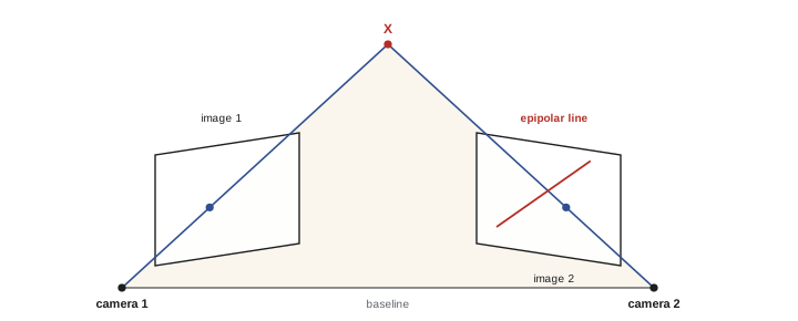
When two cameras view the same scene, a point in one image does not determine the 3D point (it could lie anywhere along its ray), but it does constrain where the matching point can appear in the other image: on a line, the epipolar line, formed by projecting that ray into the second image. All epipolar lines in an image pass through the epipole, the image of the other camera's center. For calibrated cameras, with points in normalized coordinates \(\hat{\mathbf{x}} = K^{-1}\mathbf{x}\), the constraint is expressed by the essential matrix:

where \(R\) and \(\mathbf{t}\) are the rotation and translation between the cameras and \([\mathbf{t}]_\times\) is the skew-symmetric matrix that computes cross products with \(\mathbf{t}\). For uncalibrated cameras, the same constraint in pixel coordinates uses the fundamental matrix \(F = K_2^{-\top} E K_1^{-1}\). Epipolar geometry has several uses: it reduces stereo matching to a one-dimensional search along epipolar lines (rectification makes those lines horizontal, Lesson 9), it filters wrong feature matches, and it allows the relative pose of the cameras to be recovered from matches alone.

Recovering motion and structure from two views

The essential matrix has five degrees of freedom (three for rotation and two for the direction of translation; the scale of translation cannot be determined from images alone). It can be estimated from point matches: each match gives one linear equation in the nine entries of \(E\), so eight matches determine it up to scale (the eight-point algorithm), and the five-point algorithm uses the minimum number with RANSAC (Lesson 2) to handle outliers. Decomposing \(E\) with the singular value decomposition gives four candidate pairs of \(R\) and \(\mathbf{t}\); the correct one places the triangulated points in front of both cameras.

Triangulation then finds each 3D point from its two image positions, as the point whose projections best match the observations, solved linearly (DLT) and refined by minimizing reprojection error.

import numpy as np

# Two calibrated views: estimate the essential matrix with the eight-point algorithm, then triangulate points
rng = np.random.default_rng(2)
K = np.array([[800.0, 0, 320], [0, 800.0, 240], [0, 0, 1]])
X = np.c_[rng.uniform(-2, 2, 60), rng.uniform(-1.5, 1.5, 60), rng.uniform(5, 12, 60)]   # 3D points in camera 1 frame
ang = np.radians(8)
R = np.array([[np.cos(ang), 0, np.sin(ang)], [0, 1, 0], [-np.sin(ang), 0, np.cos(ang)]])
t = np.array([-1.0, 0.0, 0.1])                         # camera 2 pose: X2 = R X1 + t

def project(P, Xw):
    x = (P @ np.c_[Xw, np.ones(len(Xw))].T).T
    return x[:, :2] / x[:, 2:]
P1 = K @ np.c_[np.eye(3), np.zeros(3)]
P2 = K @ np.c_[R, t]
x1 = project(P1, X) + rng.normal(0, 0.5, (60, 2))
x2 = project(P2, X) + rng.normal(0, 0.5, (60, 2))

Kinv = np.linalg.inv(K)
n1 = (Kinv @ np.c_[x1, np.ones(60)].T).T
n2 = (Kinv @ np.c_[x2, np.ones(60)].T).T
A = np.array([np.kron(b, a) for a, b in zip(n1, n2)])   # x2^T E x1 = 0 for each match
E = np.linalg.svd(A)[2][-1].reshape(3, 3)
U, S, Vt = np.linalg.svd(E)
E = U @ np.diag([1, 1, 0]) @ Vt                          # enforce two equal singular values and rank 2
alg = np.abs(np.sum(n2 * (n1 @ E.T), axis=1))
print(f"epipolar constraint residual |x2^T E x1|: median {np.median(alg):.2e}")
tx = np.array([[0, -t[2], t[1]], [t[2], 0, -t[0]], [-t[1], t[0], 0]])
E_true = tx @ R
c = np.sum(E * E_true) / np.linalg.norm(E) / np.linalg.norm(E_true)
print(f"agreement with the true essential matrix (|cosine|): {abs(c):.4f}")

def triangulate(a, b):
    M = np.array([a[0] * P1[2] - P1[0], a[1] * P1[2] - P1[1], b[0] * P2[2] - P2[0], b[1] * P2[2] - P2[1]])
    Xh = np.linalg.svd(M)[2][-1]
    return Xh[:3] / Xh[3]
Xe = np.array([triangulate(a, b) for a, b in zip(x1, x2)])
err = np.linalg.norm(Xe - X, axis=1)
near, far = X[:, 2] < 8, X[:, 2] >= 8
print(f"triangulation error with 0.5 px noise and a 1 m baseline: points nearer than 8 m {err[near].mean() * 100:.1f} cm, farther {err[far].mean() * 100:.1f} cm")

epipolar constraint residual |x2^T E x1|: median 3.11e-03
agreement with the true essential matrix (|cosine|): 0.9996
triangulation error with 0.5 px noise and a 1 m baseline: points nearer than 8 m 2.2 cm, farther 8.0 cm

The estimated essential matrix agrees almost perfectly with the true one despite half-pixel noise. Triangulation errors are a few centimeters and grow with distance, the same effect as in stereo depth (Lesson 9): for a fixed baseline, depth uncertainty rises roughly with the square of depth. Longer baselines give better depth but make matching harder, because the views differ more.

Pose from known points: PnP

When the 3D positions of some points are known, for example the corners of a fiducial marker, a 3D model of an object, or points in a previously built map, a camera's pose can be computed from a single image by solving the perspective-n-point (PnP) problem. Three points give up to four solutions and a fourth disambiguates; practical solvers (EPnP and others) use many points with RANSAC and refine by minimizing reprojection error. PnP is the core of marker-based augmented reality, of robot localization in a known map, and of object pose estimation for robotic grasping, where a network detects keypoints of a known object and PnP converts them to a 6-degree-of-freedom pose.

Bundle adjustment and large-scale reconstruction

Structure from motion with many images (Lesson 9) builds a reconstruction incrementally: start from a well-conditioned pair, triangulate points, add new images by PnP against the existing points, triangulate more points, and periodically refine everything with bundle adjustment. Bundle adjustment jointly optimizes all camera poses, intrinsics and 3D points to minimize the total squared reprojection error over every observation:

where \(\pi\) is the projection function and \(\rho\) a robust loss that limits the influence of remaining outliers. Problems with thousands of cameras and millions of points are solved efficiently with Levenberg-Marquardt optimization exploiting the sparse structure (each observation involves only one camera and one point). Open-source tools such as COLMAP perform the whole pipeline, and photogrammetry software is used for surveying, construction progress monitoring, heritage documentation and creating 3D content. Visual and visual-inertial SLAM (simultaneous localization and mapping) perform the same estimation in real time for robots, drones and AR headsets, fusing inertial measurements to handle fast motion and to recover scale.

Neural radiance fields and Gaussian splatting

Classical reconstruction produces point clouds and meshes, which struggle with thin structures, reflections and transparency. Neural radiance fields (NeRF, 2020) instead represent a scene as a function, learned by a neural network, mapping a 3D position and viewing direction to density and color. An image is rendered by volume rendering: for each pixel, sample points along the camera ray, query the network, and accumulate color weighted by density and transmittance:

The network is trained so that rendered images match the input photographs, whose camera poses come from structure from motion. NeRFs produce photorealistic novel views, including view-dependent effects such as reflections, but early versions took hours to train and seconds to render each image.

3D Gaussian splatting (2023) represents the scene explicitly as millions of 3D Gaussians, each with a position, shape, opacity and view-dependent color, initialized from the structure-from-motion points and optimized by rendering them as overlapping 2D splats with a fast rasterizer. It trains in minutes and renders at over 100 frames per second with quality comparable to the best NeRFs, and has quickly been adopted for virtual tours, visual effects, digital twins of buildings and sites, and real estate. Both approaches need good coverage of the scene and accurate camera poses, and they reconstruct appearance more faithfully than geometry, so surveying-grade measurements still rely on photogrammetry and lidar.

Calibrating multiple sensors

Robots and vehicles combine several cameras, lidars, radars and inertial measurement units, and fusing their data requires knowing the rigid transformation (extrinsic calibration) between every pair of sensors, and synchronizing their clocks. Camera-to-camera extrinsics come from viewing a common calibration target; camera-to-lidar calibration aligns target features visible to both, such as the edges of a board or special reflective markers, or optimizes the alignment of lidar edges with image edges in natural scenes. Calibration drifts with vibration and temperature, so vehicles monitor it online and recalibrate when residuals grow. Errors that seem small matter: a rotation error of 0.5° between a camera and a lidar shifts projected lidar points by about 44 cm at 50 m, enough to place a pedestrian's points on the wrong object.