Images and image formation

Computer vision is the field of AI that makes sense of images and video: recognizing objects, reading text, measuring shapes and distances, tracking motion and reconstructing the three-dimensional world. It powers phone cameras, medical imaging, factory inspection, driver assistance and self-driving vehicles, satellite analysis, retail checkout, document scanning and the image understanding of multimodal language models. Before a model can interpret an image, it helps to understand what an image is: how light from a scene becomes an array of numbers, what information is kept and lost, and how simple operations on those numbers reveal structure. This lesson covers image formation through the camera model, sensors and color, sampling and resolution, and the filtering operations that underlie both classical vision and convolutional neural networks. The section at the end of this lesson shows how the twelve lessons of the course fit together.

From light to pixels

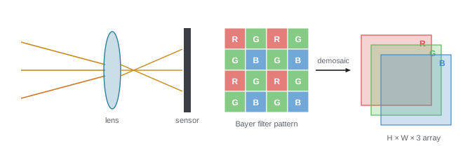
A digital camera focuses light from the scene through a lens onto an image sensor, a grid of millions of photosites (CMOS sensors in almost all modern cameras). Each photosite collects photons during the exposure and converts them to an electrical charge, which is read out and digitized, typically to 10 to 14 bits. Each photosite sees only one color: a color filter array, usually the Bayer pattern of two green, one red and one blue filter per 2 × 2 block, gives each a red, green or blue sensitivity, and demosaicing interpolates the missing colors at every pixel. The camera's image signal processor then applies white balance, noise reduction, tone mapping, sharpening and compression to produce the final image.

The result is a digital image: an array of pixels, each holding intensity values. A grayscale image of height \(H\) and width \(W\) is an \(H \times W\) matrix; a color image is an \(H \times W \times 3\) array (a tensor) of red, green and blue values, commonly stored as 8-bit integers from 0 to 255 or as floating-point numbers from 0 to 1. A 12-megapixel photo holds 36 million numbers.

Several properties of how images are stored matter for vision systems:

• Gamma encoding: pixel values in typical image files (sRGB) are not proportional to light intensity but compressed by a nonlinear curve, roughly \(V = L^{1/2.2}\), to match human perception. Physical calculations, such as blending, resizing or measuring brightness, should convert to linear values first.
• Color spaces: besides RGB, images may be represented in HSV (hue, saturation, value), useful for color-based segmentation, or YCbCr (brightness plus two color-difference channels), used by JPEG and video codecs, which store color at lower resolution than brightness because the eye is less sensitive to color detail.
• Compression: lossy formats such as JPEG discard fine detail and add block artifacts that can mislead models trained on clean data.
• Dynamic range: sensors capture a limited range of brightness; very bright areas clip and dark areas become noisy, which vision systems must handle in scenes such as tunnels and night driving.

The pinhole camera model

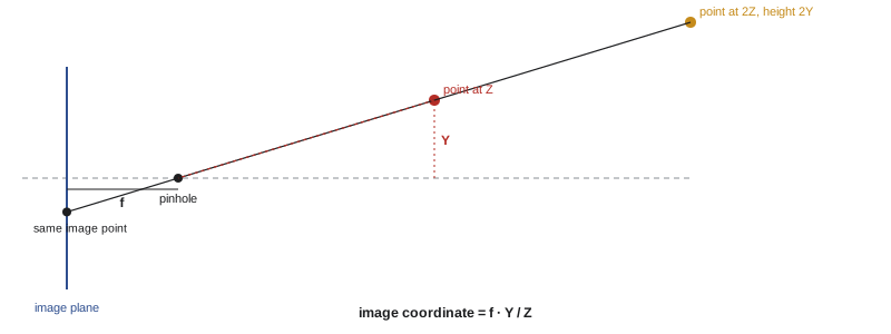
Geometric computer vision starts from the pinhole camera: light from a 3D point \((X, Y, Z)\) in camera coordinates passes through a single point (the center of projection) and lands on the image plane. By similar triangles, the image coordinates are:

where \(f_x\) and \(f_y\) are the focal length expressed in pixels and \((c_x, c_y)\) is the principal point, near the image center. In homogeneous coordinates this is a matrix multiplication by the intrinsic matrix \(K\), followed by division by depth:

A full camera model adds the extrinsic parameters, a rotation \(R\) and translation \(\mathbf{t}\) from world to camera coordinates, giving the projection \(\mathbf{x} \sim K[R\,|\,\mathbf{t}]\mathbf{X}\). Real lenses also bend straight lines (radial distortion, strongest in wide-angle and fisheye lenses), modeled with a few extra coefficients. Camera calibration estimates all these parameters by photographing a known pattern, such as a checkerboard, from several angles.

import numpy as np

# pinhole camera: focal length in pixels, principal point in the middle of the (640 x 480 image)
fx = fy = 800.0
cx, cy = 320.0, 240.0
K = np.array([[fx, 0, cx], [0, fy, cy], [0, 0, 1]])

# corners of a 1 m cube whose near face is 4 m in front of the camera (camera looks along +Z)
cube = np.array([[x, y, z] for x in (-0.5, 0.5) for y in (-0.5, 0.5) for z in (4.0, 5.0)])
uvw = (K @ cube.T).T
uv = uvw[:, :2] / uvw[:, 2:]                 # perspective division
for p, q in zip(cube, uv):
    print(f"X = {p[0]:+.1f}, Y = {p[1]:+.1f}, Z = {p[2]:.1f} m  ->  pixel ({q[0]:6.1f}, {q[1]:6.1f})")
near = uv[cube[:, 2] == 4.0]; far = uv[cube[:, 2] == 5.0]
print("near face width:", float(np.ptp(near[:, 0])), "px;  far face width:", float(np.ptp(far[:, 0])), "px")
print("horizontal field of view:", round(float(np.degrees(2 * np.arctan(320 / fx))), 1), "degrees")

X = -0.5, Y = -0.5, Z = 4.0 m  ->  pixel ( 220.0,  140.0)
X = -0.5, Y = -0.5, Z = 5.0 m  ->  pixel ( 240.0,  160.0)
X = -0.5, Y = +0.5, Z = 4.0 m  ->  pixel ( 220.0,  340.0)
X = -0.5, Y = +0.5, Z = 5.0 m  ->  pixel ( 240.0,  320.0)
X = +0.5, Y = -0.5, Z = 4.0 m  ->  pixel ( 420.0,  140.0)
X = +0.5, Y = -0.5, Z = 5.0 m  ->  pixel ( 400.0,  160.0)
X = +0.5, Y = +0.5, Z = 4.0 m  ->  pixel ( 420.0,  340.0)
X = +0.5, Y = +0.5, Z = 5.0 m  ->  pixel ( 400.0,  320.0)
near face width: 200.0 px;  far face width: 160.0 px
horizontal field of view: 43.6 degrees

The cube's near face, 4 m away, spans 200 pixels, while its far face, 1 m farther, spans 160: perspective makes distant objects smaller in proportion to their depth. Projection loses depth itself: every point along the ray through a pixel lands on the same pixel, so a single image cannot tell a small near object from a large distant one. Recovering depth requires extra information, such as a second camera, motion, known object sizes or learned priors (Lesson 9).

Sampling, resolution and aliasing

A sensor samples the continuous image projected by the lens at discrete points. The sampling theorem says that detail finer than two pixels per cycle (the Nyquist limit) cannot be represented: it either disappears or, worse, appears as a false coarser pattern called aliasing, seen as moiré on fabrics and screens. Cameras use optical low-pass filters or rely on lens blur to limit aliasing. The same issue arises when downsampling images for neural networks: shrinking an image by taking every fourth pixel aliases fine detail, so images should be blurred (low-pass filtered) or area-averaged before downsampling. Even CNNs with strided convolutions can suffer from aliasing, making them sensitive to small shifts of the input.

Filtering and convolution

Many image operations replace each pixel with a weighted sum of its neighbors. Sliding a small array of weights, the kernel or filter, across the image and computing the weighted sum at each position is convolution (strictly, cross-correlation when the kernel is not flipped, which is what deep learning libraries compute):

Different kernels perform different operations:

• Smoothing: a box filter (all weights equal) or Gaussian filter averages neighbors, reducing noise at the cost of blurring edges.
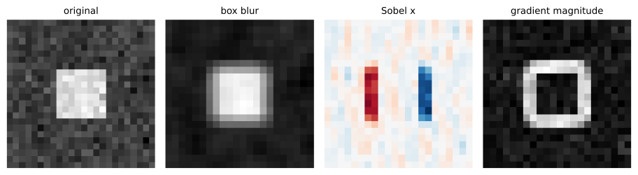
• Edge detection: derivative filters such as Sobel respond to changes in intensity. The horizontal and vertical responses \(G_x\) and \(G_y\) give the gradient magnitude \(\sqrt{G_x^2 + G_y^2}\) and direction at each pixel.
• Sharpening: subtracting a blurred version from the original enhances edges.

import numpy as np

# a synthetic 24 x 24 grayscale image: dark background, bright square, plus noise
rng = np.random.default_rng(0)
img = np.zeros((24, 24)); img[8:16, 8:16] = 1.0
img += rng.normal(0, 0.1, img.shape)

def conv2d(x, k):
    # "valid" 2-D cross-correlation, as used in CNNs
    kh, kw = k.shape
    out = np.zeros((x.shape[0] - kh + 1, x.shape[1] - kw + 1))
    for i in range(out.shape[0]):
        for j in range(out.shape[1]):
            out[i, j] = (x[i:i + kh, j:j + kw] * k).sum()
    return out

box = np.ones((3, 3)) / 9
sobel_x = np.array([[-1, 0, 1], [-2, 0, 2], [-1, 0, 1]])
smooth = conv2d(img, box)
gx, gy = conv2d(img, sobel_x), conv2d(img, sobel_x.T)
mag = np.hypot(gx, gy)

print("background noise std: original", round(float(img[:6, :6].std()), 3),
      " after 3x3 box blur", round(float(smooth[:5, :5].std()), 3))
np.set_printoptions(precision=1, suppress=True, linewidth=120)
print("gradient magnitude along row 11 (through the middle of the square):")
print(mag[10])
print("pixels with gradient magnitude > 2:", int((mag > 2).sum()), "of", mag.size)

background noise std: original 0.087  after 3x3 box blur 0.033
gradient magnitude along row 11 (through the middle of the square):
[0.3 0.6 0.5 0.3 0.5 0.6 3.4 3.1 0.2 0.4 0.5 0.4 0.5 0.4 3.9 4.1 0.2 0.2 0.7 0.1 0.4 0.4]
pixels with gradient magnitude > 2: 60 of 484

Averaging nine pixels with independent noise reduces the noise standard deviation by about a factor of three (\(\sqrt9\)), from 0.087 to 0.033. The Sobel gradient is near zero in flat regions and around 3 to 4 where the bright square meets the background, so thresholding it finds the square's outline. Edges are informative because object boundaries, texture and shape show up as intensity changes, and early layers of trained CNNs learn filters that look much like these hand-designed edge and blob detectors.

Classical features and the shift to learning

Before deep learning, vision systems used hand-designed features computed from gradients and filters. Corner detectors (Harris) found points that could be matched across images; SIFT (2004) described the gradient pattern around keypoints in a way robust to scale and rotation, enabling panorama stitching and 3D reconstruction; histograms of oriented gradients (HOG, 2005) combined with linear classifiers detected pedestrians. These features worked well for matching and for some recognition tasks, but designing features for every object category was impractical. In 2012, AlexNet, a convolutional neural network trained on 1.2 million labeled ImageNet images with GPUs, cut the ImageNet classification error from about 26% to 15%, and learned features rapidly replaced hand-designed ones. Lesson 3 explains how CNNs learn their own filters.

Classical techniques remain useful: filtering and edge detection for preprocessing and simple inspection tasks, camera calibration and geometry for measurement and 3D (Lessons 9 and 10), and keypoint matching in robotics and mapping. Understanding them also makes it easier to see what neural networks learn and where they fail.

How this course is organized

The twelve lessons move from pixels to deployed systems:

• Lesson 1 (this lesson): image formation, the pinhole camera, sensors, sampling and convolution.
• Lesson 2: image processing, features, homographies and RANSAC.
• Lesson 3: convolutional neural networks, architectures, training and transfer learning.
• Lesson 4: efficient networks, datasets, evaluation and calibration.
• Lesson 5: object detection and segmentation, IoU, NMS and average precision.
• Lesson 6: inside modern detectors: assignment, focal loss, DETR, panoptic segmentation and pose.
• Lesson 7: vision transformers, self-supervised learning and CLIP.
• Lesson 8: generative models for images and video.
• Lesson 9: video, tracking, stereo and 3D vision.
• Lesson 10: multiple-view geometry, calibration and 3D reconstruction.
• Lesson 11: vision-language models and document understanding.
• Lesson 12: deploying vision systems, robustness, privacy and a capstone project.