Efficient networks, evaluation and calibration

Lesson 3 explained how convolutional networks are built and trained, and how transfer learning makes them practical with modest data. Building a vision system that works in the field requires more: choosing an architecture that fits the device and latency budget, assembling and splitting datasets so that evaluation is honest, measuring performance in ways that match the application, making the model's confidence trustworthy, handling rare classes and anomalies, and checking that the model keeps working when the cameras, lighting or population change. This lesson covers efficient architectures for edge devices, dataset practice, evaluation metrics for classification, calibration, class imbalance and anomaly detection, and robustness testing.

Efficient architectures

Many vision models run on phones, cameras, drones, vehicles and factory controllers with limited compute, memory and power, often within a strict latency budget such as 33 ms per frame for 30 frames per second. Efficient architectures reduce computation with a few key ideas:

• Depthwise separable convolutions (MobileNet, 2017) split a standard convolution into a depthwise convolution, which filters each channel separately with its own \(k \times k\) kernel, and a pointwise 1 × 1 convolution, which mixes channels. For a 3 × 3 kernel this cuts computation by about 8 to 9 times with a modest loss of accuracy.
• Inverted residual blocks with linear bottlenecks (MobileNetV2) expand channels, apply a depthwise convolution, and project back down, with a residual connection.
• Compound scaling (EfficientNet, 2019) scales depth, width and input resolution together by fixed ratios, rather than one at a time, giving better accuracy for a given compute budget.
• Neural architecture search automates the search for efficient designs on a target device.

# Parameters and multiply-accumulate operations (MACs): standard versus depthwise separable convolution
def standard(h, w, cin, cout, k):
    params = k * k * cin * cout
    return params, params * h * w

def separable(h, w, cin, cout, k):
    dw = k * k * cin                  # depthwise: one k x k filter per input channel
    pw = cin * cout                   # pointwise: 1 x 1 convolution mixing channels
    return dw + pw, (dw + pw) * h * w

for h, cin, cout in ((112, 32, 64), (56, 128, 128), (14, 512, 512), (7, 1024, 1024)):
    p1, m1 = standard(h, h, cin, cout, 3)
    p2, m2 = separable(h, h, cin, cout, 3)
    print(f"{h:3d}x{h:<3d} {cin:4d}->{cout:<4d}: standard {p1 / 1e3:7.1f}k params {m1 / 1e6:7.1f}M MACs | separable {p2 / 1e3:6.1f}k params {m2 / 1e6:6.1f}M MACs | {m1 / m2:4.1f}x fewer")
# Rough latency on a device sustaining 200 GMAC/s with 30% utilization, for whole networks
for name, gmacs in (("ResNet-50", 4.1), ("MobileNetV2", 0.30), ("EfficientNet-B0", 0.39), ("ViT-B/16", 17.6)):
    print(f"{name:16s} {gmacs:5.2f} GMACs per image -> about {gmacs / (200 * 0.3) * 1000:6.1f} ms per image")

112x112   32->64  : standard    18.4k params   231.2M MACs | separable    2.3k params   29.3M MACs |  7.9x fewer
 56x56   128->128 : standard   147.5k params   462.4M MACs | separable   17.5k params   55.0M MACs |  8.4x fewer
 14x14   512->512 : standard  2359.3k params   462.4M MACs | separable  266.8k params   52.3M MACs |  8.8x fewer
  7x7   1024->1024: standard  9437.2k params   462.4M MACs | separable 1057.8k params   51.8M MACs |  8.9x fewer
ResNet-50         4.10 GMACs per image -> about   68.3 ms per image
MobileNetV2       0.30 GMACs per image -> about    5.0 ms per image
EfficientNet-B0   0.39 GMACs per image -> about    6.5 ms per image
ViT-B/16         17.60 GMACs per image -> about  293.3 ms per image

Depthwise separable layers need about 8 to 9 times fewer operations and parameters. Whole-network compute differs by more than an order of magnitude between MobileNetV2 and ResNet-50, and by more again for a ViT-Base, which is why mobile and embedded systems use efficient CNNs or small, distilled transformers. These latency figures are only rough guides: real speed depends on memory bandwidth, how well the operations map to the hardware, batch size and the runtime, so models should be benchmarked on the target device. Quantizing to 8-bit integers, pruning and knowledge distillation (AI-340, Lesson 10) reduce cost further, and runtimes such as TensorRT, Core ML, TensorFlow Lite and ONNX Runtime optimize models for specific hardware.

Building datasets

Data quality usually matters more than architecture. Good practice for vision datasets:

• Cover the real conditions: cameras, viewpoints, lighting, weather, seasons, backgrounds and object variations that the deployed system will see, including rare but important cases.
• Write clear labeling guidelines with examples of edge cases, measure agreement between annotators, and review a sample of labels. Label noise of a few percent is common in large datasets and can be found by examining training examples the model gets confidently wrong.
• Split data so that evaluation is honest. Images from the same video, patient, product batch, location or day are highly correlated; if some go to training and others to testing, the test score is inflated. Split by these groups, not by individual images, and remove near-duplicates across splits.
• Keep a held-out test set that is not used for any decision during development, and a separate validation set for model selection and tuning.
• Document the dataset: sources, collection dates, consent, demographics where relevant, labeling process and known limitations (datasheets for datasets).

Evaluating classifiers

Accuracy alone can mislead, especially with imbalanced classes: a defect detector that always predicts "good" is 99% accurate if 1% of parts are defective. Better tools:

• The confusion matrix, counting predictions against true classes, shows which classes are confused with which.
• Precision, recall and F1 for each class (AI-210), and their macro-average across classes, which weights rare classes equally.
• Top-5 accuracy for problems with many similar classes, such as ImageNet's 1,000 categories.
• ROC and precision-recall curves, and the area under them, for binary decisions with an adjustable threshold. In screening applications, the threshold is chosen for a target sensitivity (recall) or false positive rate rather than maximum accuracy.
• Performance by subgroup: camera, site, lighting condition, skin tone, age group. Aggregate metrics can hide poor performance on important subgroups.
• Confidence intervals, from bootstrap resampling of the test set, so that small differences between models are not over-interpreted.

Calibration

A classifier is calibrated if its confidence matches its accuracy: among all predictions made with 80% confidence, about 80% should be correct. Calibration matters whenever decisions use the confidence, for example to send uncertain cases to a person, to combine model outputs with other evidence, or to report risk to a doctor. Modern deep networks are often overconfident, because training drives the cross-entropy loss down by inflating logits. Calibration is measured with a reliability diagram, plotting accuracy against confidence in bins, and summarized by the expected calibration error:

Temperature scaling, the simplest and most effective fix, divides all logits by a single temperature \(T > 1\) learned on a validation set by minimizing the negative log-likelihood. It softens the probabilities without changing which class is predicted, so accuracy is unchanged.

import numpy as np

# Calibration: expected calibration error (ECE) before and after temperature scaling
rng = np.random.default_rng(0)
n, K = 5000, 10
true = rng.integers(0, K, n)
logits = rng.normal(0, 1, (n, K))
logits[np.arange(n), true] += rng.normal(2.2, 1.2, n)     # signal toward the true class
logits *= 3.0                                              # an overconfident network: logits too large

def softmax(z):
    z = z - z.max(axis=1, keepdims=True)
    e = np.exp(z)
    return e / e.sum(axis=1, keepdims=True)

def ece(p, y, bins=15):
    conf = p.max(axis=1); pred = p.argmax(axis=1); acc = pred == y
    edges = np.linspace(0, 1, bins + 1); total = 0.0
    for a, b in zip(edges[:-1], edges[1:]):
        m = (conf > a) & (conf <= b)
        if m.any():
            total += m.mean() * abs(acc[m].mean() - conf[m].mean())
    return total, acc.mean(), conf.mean()

val, test = np.arange(0, 2500), np.arange(2500, n)
def nll(T, idx):
    p = softmax(logits[idx] / T)
    return -np.log(p[np.arange(len(idx)), true[idx]] + 1e-12).mean()
Ts = np.linspace(0.5, 5, 451)
T_best = Ts[np.argmin([nll(T, val) for T in Ts])]
for T, label in ((1.0, "uncalibrated"), (T_best, f"temperature T = {T_best:.2f}")):
    e, acc, conf = ece(softmax(logits[test] / T), true[test])
    print(f"{label:22s}: accuracy {acc:.3f}, mean confidence {conf:.3f}, ECE {e:.3f}")

uncalibrated          : accuracy 0.666, mean confidence 0.810, ECE 0.144
temperature T = 1.92  : accuracy 0.666, mean confidence 0.644, ECE 0.038

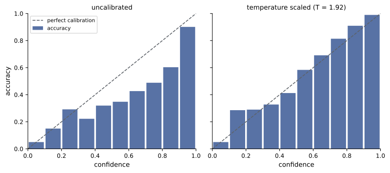
The uncalibrated model claims 81% average confidence but is right only 67% of the time; after temperature scaling with \(T \approx 1.9\), confidence and accuracy nearly match and the ECE falls from 0.14 to 0.04. Calibration should be checked again after deployment, because distribution shift typically makes models overconfident on unfamiliar inputs.

Imbalanced classes and rare defects

Many vision problems are severely imbalanced: defects, diseases, safety incidents and wildlife sightings are rare. Techniques to cope:

• Collect more rare examples deliberately, and use augmentation or synthetic data (rendered 3D models, copy-paste of defects onto good images, generative models, Lesson 8).
• Reweight the loss by class frequency, oversample rare classes, or use the focal loss (Lesson 6), which down-weights easy examples.
• Choose the decision threshold for the required recall, not 0.5.
• Evaluate with per-class recall, precision-recall curves and costs that reflect the consequences of each error type.

When defects are so rare or varied that they cannot be collected, anomaly detection learns only what normal looks like and flags anything different. Approaches include autoencoders that reconstruct normal images well and anomalies poorly, and methods that compare features of a test image with a memory bank of features from normal images (for example PatchCore), which localize anomalies to image patches. Anomaly detection is widely used in manufacturing inspection, where a few hundred images of good parts may be all that is available at launch.

Robustness and distribution shift

Models fail when deployment conditions differ from training conditions, a problem called distribution shift: new cameras with different color processing, a different lens or resolution, seasonal changes, dirty lenses, motion blur, new product variants, or a different patient population. Benchmarks such as ImageNet-C (corruptions such as noise, blur, fog and JPEG compression) and ImageNet-R (renditions such as paintings and cartoons) show that accuracy can fall dramatically under such shifts. Practical defenses:

• Collect training data from the deployment environment and update it over time.
• Use augmentation that simulates expected corruptions: blur, noise, compression, brightness and color changes.
• Start from large, diverse pretrained models, which are generally more robust (Lesson 7).
• Test explicitly on held-out sites, cameras and conditions before deployment, and monitor input statistics and prediction confidence in production to detect drift.
• Design the system so that uncertain predictions are routed to people, and so that failures are safe.