Convolutional neural networks

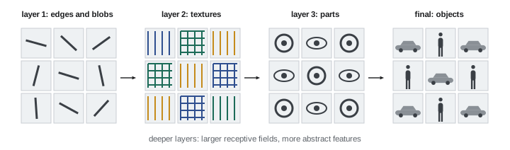
Convolutional neural networks (CNNs) brought computer vision its first great leap in the deep learning era. Instead of hand-designing filters, a CNN learns them from data: early layers learn edge and color detectors, middle layers learn textures and parts, and deep layers respond to whole objects. CNNs dominated vision from 2012 to about 2020 and remain widely used, especially where efficiency matters, as on phones, cameras and embedded devices. This lesson explains the convolutional layer and why it suits images, how output sizes, parameters and receptive fields are calculated, the architectures that shaped the field, how CNNs are trained and adapted to new tasks, and their weaknesses.

Why convolution suits images

A fully connected layer connects every input value to every output unit. For images this is wasteful and ignores structure: a 224 × 224 × 3 image has 150,528 values, so even 64 fully connected units need nearly 10 million weights. Convolutional layers build in three assumptions that match images:

• Locality: useful features, such as edges and corners, depend on nearby pixels, so each output looks only at a small neighborhood (its receptive field).
• Weight sharing: the same feature can appear anywhere, so the same filter weights are applied at every position, drastically reducing parameters.
• Translation equivariance: shifting the input shifts the feature map by the same amount, so a feature is detected wherever it occurs. Pooling and global averaging then add some translation invariance, so that classification does not depend on exact position.

These assumptions are an inductive bias: they let CNNs learn from far less data than a fully connected network would need, at the cost of limiting what patterns are easy to represent.

The convolutional layer

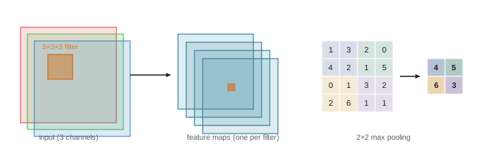
A convolutional layer takes an input of \(C_{in}\) channels (3 for an RGB image; many more in deeper layers) and applies \(C_{out}\) filters, each of size \(k \times k \times C_{in}\), producing \(C_{out}\) feature maps. Each filter has \(k^2 C_{in}\) weights plus a bias, so the layer has:

Stride \(s\) moves the filter several pixels at a time, reducing resolution; padding \(p\) adds zeros around the border so edge pixels are covered. The output size is:

An activation function, almost always ReLU (\(\max(0, x)\)) or a smooth variant, follows each convolution. Pooling layers downsample feature maps by taking the maximum (max pooling) or average over small windows, typically 2 × 2 with stride 2, halving width and height. As the network deepens, spatial resolution falls and the number of channels grows, trading "where" information for "what" information.

Receptive field

Each output unit of a layer depends on a region of the input image, its receptive field. Stacking layers grows the receptive field: two 3 × 3 convolutions see 5 × 5, three see 7 × 7, and strided layers and pooling multiply the growth. Deep units need large receptive fields to recognize whole objects. The receptive field \(r\) grows by \((k - 1) \times j\) at each layer, where \(j\) is the product of the strides of all earlier layers.

def conv_out(n, k, s=1, p=0):
    return (n + 2 * p - k) // s + 1

# a small CNN for 224 x 224 RGB images: (name, kernel, stride, padding, output channels); "pool" halves the size
layers = [("conv1", 7, 2, 3, 64), ("pool", 3, 2, 1, None), ("conv2", 3, 1, 1, 128),
          ("conv3", 3, 2, 1, 256), ("conv4", 3, 2, 1, 512)]
n, c = 224, 3
rf, jump = 1, 1                            # receptive field and spacing between output pixels
total = 0
for name, k, s, p, out_c in layers:
    n = conv_out(n, k, s, p)
    rf += (k - 1) * jump
    jump *= s
    params = 0 if out_c is None else k * k * c * out_c + out_c
    macs = 0 if out_c is None else n * n * k * k * c * out_c
    total += params
    c = c if out_c is None else out_c
    print(f"{name:5s}: output {n:3d} x {n:3d} x {c:3d}  params {params:9,d}  MACs {macs / 1e6:7.1f} M  receptive field {rf:3d} px")
print(f"total conv parameters: {total:,d}")
print(f"a fully connected layer from the 224 x 224 x 3 input to just 64 units would need {224 * 224 * 3 * 64:,d} weights")

conv1: output 112 x 112 x  64  params     9,472  MACs   118.0 M  receptive field   7 px
pool : output  56 x  56 x  64  params         0  MACs     0.0 M  receptive field  11 px
conv2: output  56 x  56 x 128  params    73,856  MACs   231.2 M  receptive field  19 px
conv3: output  28 x  28 x 256  params   295,168  MACs   231.2 M  receptive field  27 px
conv4: output  14 x  14 x 512  params 1,180,160  MACs   231.2 M  receptive field  43 px
total conv parameters: 1,558,656
a fully connected layer from the 224 x 224 x 3 input to just 64 units would need 9,633,792 weights

A first 7 × 7 convolution with stride 2 and a stride-2 pooling quickly reduce the 224 × 224 image to 56 × 56, and by the fourth convolution each unit sees a 43-pixel region of the input, enough for object parts. Deeper networks continue this growth until units see most of the image. The whole stack has 1.6 million parameters, far fewer than a single fully connected layer of 64 units on the raw input (9.6 million), yet each convolution layer performs over 100 million multiply-adds.

Landmark architectures

A sequence of architectures defined the field:

• LeNet-5 (1998): Yann LeCun's network for reading handwritten digits on checks, with two convolution and pooling stages, already containing the key ideas.
• AlexNet (2012): eight layers, ReLU activations, dropout and GPU training, winning ImageNet by a wide margin.
• VGG (2014): showed that stacks of simple 3 × 3 convolutions, 16 to 19 layers deep, work well.
• GoogLeNet/Inception (2014): parallel filters of several sizes and 1 × 1 convolutions to reduce computation.
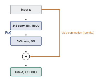
• ResNet (2015): residual connections, in which each block learns a correction added to its input (\(\mathbf{y} = \mathbf{x} + F(\mathbf{x})\)), allowed training networks of 50 to over 100 layers by giving gradients a direct path, and won ImageNet with 3.6% top-5 error, below estimated human performance on that benchmark. Residual connections are now used in almost every deep architecture, including transformers.
• Batch normalization (2015) normalizes activations within each mini-batch, stabilizing and speeding training.
• Efficient designs: MobileNet (depthwise separable convolutions) and EfficientNet (balanced scaling of depth, width and resolution) for phones and embedded devices.
• ConvNeXt (2022): modernized CNNs with design ideas from vision transformers, showing CNNs remain competitive at scale.

Training CNNs

CNNs for classification end with global average pooling and a fully connected layer producing one score (logit) per class, followed by softmax, and are trained by minimizing cross-entropy loss with stochastic gradient descent or Adam (AI-310). Practical training depends on:

• Data augmentation: random crops, flips, color jitter, rotations and more aggressive methods (mixup, cutout, RandAugment) create varied copies of training images, teaching invariances the architecture alone does not provide and reducing overfitting.
• Normalization and regularization: batch normalization, weight decay, dropout and label smoothing.
• Learning-rate schedules: warm-up followed by cosine or step decay.

The following experiment shows the effect of convolution, pooling and augmentation on robustness to small shifts, using the 8 × 8 handwritten digits dataset. To keep it fast, the convolutional filters are random rather than learned; only the final classifier is trained.

import numpy as np
from sklearn.datasets import load_digits
from sklearn.linear_model import LogisticRegression

digits = load_digits()                      # 1797 handwritten digits, 8 x 8 pixels
X = digits.images / 16.0; y = digits.target
rng = np.random.default_rng(0)
idx = rng.permutation(len(y)); tr, te = idx[:1300], idx[1300:]

def shift(imgs, dx):
    # move every image dx pixels to the right, filling with zeros
    out = np.zeros_like(imgs)
    out[:, :, dx:] = imgs[:, :, :8 - dx] if dx > 0 else imgs
    return out

filters = rng.normal(0, 1, (16, 3, 3))      # 16 random 3 x 3 filters (not trained)
def conv_features(imgs):
    n = len(imgs)
    maps = np.zeros((n, 16, 6, 6))
    for i in range(6):
        for j in range(6):
            patch = imgs[:, i:i + 3, j:j + 3]
            maps[:, :, i, j] = np.einsum("nab,fab->nf", patch, filters)
    maps = np.maximum(maps, 0)              # ReLU
    pooled = maps.reshape(n, 16, 3, 2, 3, 2).max(axis=(3, 5))   # 2 x 2 max pooling -> 3 x 3
    return pooled.reshape(n, -1)

raw = LogisticRegression(max_iter=3000).fit(X[tr].reshape(len(tr), -1), y[tr])
cnn = LogisticRegression(max_iter=3000).fit(conv_features(X[tr]), y[tr])
# data augmentation: train the conv model on copies shifted by 0, 1 and 2 pixels
Xa = np.concatenate([shift(X[tr], d) for d in (0, 1, 2)]); ya = np.tile(y[tr], 3)
aug = LogisticRegression(max_iter=3000).fit(conv_features(Xa), ya)
print("shift   raw pixels   conv features   conv + augmentation")
for dx in (0, 1, 2):
    Xt = shift(X[te], dx)
    a_raw = raw.score(Xt.reshape(len(te), -1), y[te])
    a_cnn = cnn.score(conv_features(Xt), y[te])
    a_aug = aug.score(conv_features(Xt), y[te])
    print(f"{dx} px     {a_raw:.3f}        {a_cnn:.3f}           {a_aug:.3f}")

shift   raw pixels   conv features   conv + augmentation
0 px     0.978        0.988           0.970
1 px     0.419        0.628           0.976
2 px     0.064        0.137           0.962

All three models classify unshifted test digits well (97 to 99%). Shifting the test digits by a single pixel collapses the raw-pixel model to 42% and a 2-pixel shift to 6%, because it learned weights tied to exact pixel positions. Convolution with ReLU and max pooling helps somewhat (63% at 1 pixel), since pooling tolerates small movements within each pooling window. Training with shifted copies (augmentation) makes the model robust: 97% and 96% on shifted digits. Architecture provides some invariance; data and augmentation provide most of it.

Transfer learning

Training a large CNN from scratch needs millions of labeled images. Most practical applications instead start from a network pretrained on a large dataset such as ImageNet and adapt it:

• Feature extraction: freeze the pretrained layers and train only a new final classifier on the target data. Works with a few hundred images per class.
• Fine-tuning: continue training some or all layers at a low learning rate, usually better with a few thousand images.

Transfer works because early and middle layers learn general features (edges, textures, shapes) useful for almost any visual task. It has made vision practical in fields with little labeled data, such as medical imaging, agriculture and industrial inspection. Increasingly, the starting point is a large self-supervised or vision-language model rather than an ImageNet classifier (Lesson 7).

Understanding and trusting CNNs

CNNs are accurate but opaque. Several tools help reveal what they use:

• Saliency maps show which pixels most affect the output, through gradients of the class score with respect to the input.
• Class activation maps, such as Grad-CAM, highlight the image regions that contributed to a class by weighting the last convolutional feature maps by their gradients.
• Feature visualization optimizes an input to maximally activate a neuron, revealing the patterns it detects.

These tools have exposed shortcut learning: models that classify correctly for the wrong reasons, such as a pneumonia detector that learned hospital-specific markers in X-rays, or a classifier that recognized cows mostly from green pastures. CNNs also rely more on texture than shape compared with humans, are vulnerable to adversarial examples (tiny, carefully crafted pixel changes that flip predictions), and degrade under distribution shift such as new cameras, weather or lighting. Testing on data from the deployment environment, and on deliberately varied conditions, is essential.

Lesson 4 continues with efficient architectures for edge devices, honest dataset splits, evaluation metrics and calibration.