Graphical models

A probabilistic model of a realistic problem involves many variables: symptoms and diseases, words and topics, pixels and objects, sensor readings and hidden machine states. Writing down their joint distribution directly is hopeless. Twenty binary variables already have \(2^{20} - 1\), about a million, free probabilities, and inference by summing over the table is equally impossible. Graphical models make large models tractable by exploiting structure: most variables interact directly with only a few others. A graph records which variables depend directly on which, the joint distribution factorizes accordingly, and inference algorithms work on the graph. This lesson covers directed models (Bayesian networks), conditional independence and d-separation, undirected models, exact inference by variable elimination and message passing, and hidden Markov models as a worked example.

Bayesian networks

A Bayesian network is a directed acyclic graph (DAG) whose nodes are random variables, together with a conditional distribution for each node given its parents. The joint distribution is the product of these local conditionals:

The chain rule of probability always allows a joint distribution to be written as a product of conditionals, \(p(x_1)p(x_2 \mid x_1)p(x_3 \mid x_1, x_2)\cdots\). The graph's contribution is to drop most of the conditioning variables, asserting that each variable depends directly only on its parents. That assertion is what saves parameters and computation.

A classic small example concerns a wet lawn. Cloudy weather (C) makes rain (R) more likely and makes it less likely that the sprinkler (S) is switched on; both rain and the sprinkler can make the grass wet (W). The joint distribution factorizes as \(p(C)\,p(S \mid C)\,p(R \mid C)\,p(W \mid S, R)\). With binary variables, the full table needs 15 free numbers; the network needs \(1 + 2 + 2 + 4 = 9\). For large networks, the saving is exponential: a node with \(k\) binary parents needs \(2^k\) numbers, so a network in which every node has at most three parents grows linearly with the number of nodes rather than exponentially.

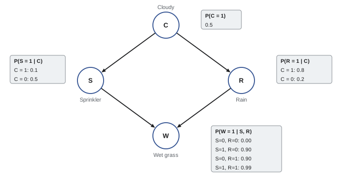
Bayesian networks are often built from causal knowledge, drawing arrows from causes to effects, which makes them easy for domain experts to specify and interpret. Strictly, though, a Bayesian network encodes only conditional independence; giving the arrows a causal meaning, so that the network predicts the effect of interventions, is an additional assumption studied in causal inference.

Inference by enumeration

Inference means computing the distribution of some variables given observed values of others, such as \(P(R = 1 \mid W = 1)\): given that the grass is wet, how likely is it that it rained? The direct method sums the joint distribution over all unobserved variables, then normalizes.

import itertools

pC = {1: 0.5, 0: 0.5}
pS = {1: {1: 0.1, 0: 0.9}, 0: {1: 0.5, 0: 0.5}}          # pS[c][s]
pR = {1: {1: 0.8, 0: 0.2}, 0: {1: 0.2, 0: 0.8}}          # pR[c][r]
pW1 = {(0, 0): 0.0, (1, 0): 0.9, (0, 1): 0.9, (1, 1): 0.99}  # P(W=1 | s, r)

def joint(c, s, r, w):
    pw = pW1[(s, r)] if w == 1 else 1 - pW1[(s, r)]
    return pC[c] * pS[c][s] * pR[c][r] * pw

def prob(query, evidence):
    num = den = 0.0
    for c, s, r, w in itertools.product([0, 1], repeat=4):
        x = dict(C=c, S=s, R=r, W=w)
        if all(x[k] == v for k, v in evidence.items()):
            p = joint(c, s, r, w)
            den += p
            if all(x[k] == v for k, v in query.items()):
                num += p
    return num / den

print(f"P(R=1)             = {prob(dict(R=1), dict()):.3f}")
print(f"P(R=1 | W=1)       = {prob(dict(R=1), dict(W=1)):.3f}")
print(f"P(R=1 | W=1, S=1)  = {prob(dict(R=1), dict(W=1, S=1)):.3f}")
print(f"P(S=1 | W=1)       = {prob(dict(S=1), dict(W=1)):.3f}")
print(f"P(S=1 | W=1, R=1)  = {prob(dict(S=1), dict(W=1, R=1)):.3f}")

P(R=1)             = 0.500
P(R=1 | W=1)       = 0.708
P(R=1 | W=1, S=1)  = 0.320
P(S=1 | W=1)       = 0.430
P(S=1 | W=1, R=1)  = 0.194

Observing wet grass raises the probability of rain from 0.5 to about 0.71. Learning that the sprinkler was on then lowers it again, to about 0.32: the sprinkler explains the wet grass, so rain is no longer needed as an explanation. Likewise, learning that it rained lowers the probability that the sprinkler was on. This pattern, in which two causes of a common effect become dependent once the effect is observed, is called explaining away. It is one of the reasoning patterns that graphical models capture naturally and that simple rule-based systems get wrong.

Conditional independence and d-separation

The graph structure implies conditional independence relationships that hold for any choice of the conditional probability tables. They follow from three basic patterns of three nodes:

• Chain, \(A \to B \to C\): \(A\) and \(C\) are dependent, but independent given \(B\). Observing the middle variable blocks the flow of information.
• Fork (common cause), \(A \leftarrow B \to C\): \(A\) and \(C\) are dependent, because they share a cause, but independent given \(B\). Ice cream sales and drownings are correlated through summer weather; given the weather, they are not.
• Collider (common effect), \(A \to B \leftarrow C\): \(A\) and \(C\) are independent, but become dependent given \(B\), or given any descendant of \(B\). This is explaining away; it is also the source of selection bias, such as Berkson's paradox, in which conditioning on admission to a hospital creates a spurious negative correlation between two unrelated diseases.

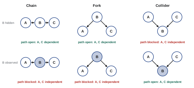
D-separation extends these rules to whole graphs. A path between two nodes is blocked by a set of observed nodes \(Z\) if it contains a chain or fork whose middle node is in \(Z\), or a collider whose middle node is not in \(Z\) and has no descendant in \(Z\). If every path between \(X\) and \(Y\) is blocked, then \(X\) and \(Y\) are d-separated by \(Z\), and they are conditionally independent given \(Z\) in every distribution that factorizes according to the graph.

A useful consequence is the Markov blanket: a node is conditionally independent of all other nodes given its parents, its children and its children's other parents. Only the Markov blanket matters when updating one variable, which is what makes Gibbs sampling (Lesson 7) efficient on graphical models.

Undirected models: Markov random fields

Some dependencies have no natural direction: neighboring pixels in an image, adjacent atoms in a magnetic material, or words that tend to co-occur. A Markov random field (MRF) uses an undirected graph and defines the joint distribution as a normalized product of non-negative potential functions over the cliques (fully connected subsets) of the graph:

Potentials are not probabilities; they express compatibility, with larger values for configurations that are more likely. Writing \(\psi_c = \exp(-E_c)\) gives the energy-based form \(p(\mathbf x) \propto \exp(-E(\mathbf x))\). The Ising model, with binary spins on a grid and an energy that rewards neighbors agreeing, is the classic MRF; image denoising models use the same structure to prefer smooth images. Conditional independence in an MRF is simpler than in a Bayesian network: two sets of nodes are independent given a third if every path between them passes through the third.

The normalizing constant \(Z\), the partition function, is a sum over all configurations and is generally intractable. This makes learning MRF parameters harder than learning Bayesian network tables, which can be estimated by counting. Conditional random fields (CRFs), which model \(p(\mathbf y \mid \mathbf x)\) as an MRF over labels \(\mathbf y\) given inputs \(\mathbf x\), were the standard model for sequence labeling before neural sequence models and are still used as output layers on top of them.

Both directed and undirected models can be converted to factor graphs, bipartite graphs with one node per variable and one node per factor, connected when the factor involves the variable. Factor graphs are the natural setting for the message-passing algorithms below.

Exact inference

Variable elimination

Enumeration costs time exponential in the number of variables. Variable elimination does much better by pushing sums inside the product and summing out one variable at a time. For a chain \(A \to B \to C \to D\), the marginal of \(D\) is

Computing the innermost sum gives a table over \(b\), which is then used in the next sum, and so on: each step costs \(k^2\) operations for variables with \(k\) states, so the chain costs \(O(nk^2)\) instead of \(O(k^n)\). In a general graph, summing out a variable creates a new factor over all its neighbors, and the cost depends on the largest such factor created. The best possible elimination order gives a cost exponential in the treewidth of the graph. Trees and chains have treewidth 1 and are easy; grids and densely connected graphs have large treewidth, and exact inference becomes intractable. In general, exact inference in Bayesian networks is NP-hard, which motivates the approximate methods of Lessons 7 and 9.

import numpy as np

rng = np.random.default_rng(0)
n, k = 10, 4                                   # chain of 10 variables with 4 states each
p0 = rng.dirichlet(np.ones(k))
T = [rng.dirichlet(np.ones(k), size=k) for _ in range(n - 1)]   # T[i][a, b] = p(x_{i+1}=b | x_i=a)

# variable elimination: push the sums inward, one variable at a time
msg = p0.copy()
ops_ve = 0
for t in T:
    msg = msg @ t
    ops_ve += k * k
print("marginal of last variable (elimination):", np.round(msg, 4))

# brute force: build the full joint table over all 4**10 configurations
joint = p0.copy()
for t in T:
    joint = joint[..., None] * t.reshape((1,) * (joint.ndim - 1) + (k, k))
brute = joint.reshape(-1, k).sum(axis=0)
print("marginal of last variable (brute force):", np.round(brute, 4))
print(f"table entries: elimination {ops_ve}, brute force {k ** n:,}")

marginal of last variable (elimination): [0.149  0.3362 0.1665 0.3483]
marginal of last variable (brute force): [0.149  0.3362 0.1665 0.3483]
table entries: elimination 144, brute force 1,048,576

Belief propagation

On a tree-structured graph, all marginals can be computed at once by passing messages along the edges. The message from node \(i\) to neighbor \(j\) summarizes everything on \(i\)'s side of the edge:

where \(\phi_i\) is the local evidence at node \(i\). After messages have passed from the leaves to a root and back, each node's marginal is proportional to its local evidence times all incoming messages. This sum-product algorithm costs twice a single variable elimination but delivers every marginal. Replacing sums by maximizations gives the max-product algorithm, which finds the most probable joint configuration. On graphs with cycles, the same updates can be iterated anyway; this loopy belief propagation is not guaranteed to converge or to be exact, but it works remarkably well in some applications, notably the decoding of turbo and LDPC error-correcting codes used in mobile and Wi-Fi communication.

Hidden Markov models

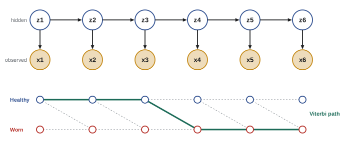
A hidden Markov model (HMM) is a Bayesian network for sequences. A hidden state \(z_t\) evolves as a Markov chain with transition matrix \(A_{ij} = p(z_{t+1} = j \mid z_t = i)\), and at each step emits an observation \(x_t\) with distribution \(p(x_t \mid z_t)\). The joint distribution is

HMMs model speech (hidden phonemes, observed acoustics), gene sequences (hidden coding regions, observed bases), machine condition monitoring (hidden health states, observed vibration levels) and many other sequential problems. The graph is a chain, so exact inference is efficient. The forward algorithm computes \(\alpha_t(j) = p(x_1, \ldots, x_t, z_t = j)\) recursively, \(\alpha_{t+1}(j) = p(x_{t+1} \mid j)\sum_i \alpha_t(i)A_{ij}\), giving the likelihood of the whole sequence in \(O(TK^2)\) time for \(K\) states. A backward pass gives the smoothed marginals \(p(z_t \mid \mathbf x)\), and the Viterbi algorithm, the max-product version, finds the most probable state sequence.

import numpy as np

# Machine health: state 0 = healthy, 1 = worn. Observation: vibration level 0 = low, 1 = medium, 2 = high.
pi = np.array([0.95, 0.05])
A = np.array([[0.90, 0.10],
              [0.00, 1.00]])                 # wear does not repair itself
B = np.array([[0.70, 0.25, 0.05],            # B[state, observation]
              [0.10, 0.40, 0.50]])
x = [0, 0, 1, 0, 1, 2, 1, 2, 2]

# forward algorithm with scaling, giving filtered probabilities p(z_t | x_1..t)
alpha = pi * B[:, x[0]]
loglik = np.log(alpha.sum()); alpha /= alpha.sum()
filtered = [alpha[1]]
for obs in x[1:]:
    alpha = (alpha @ A) * B[:, obs]
    loglik += np.log(alpha.sum()); alpha /= alpha.sum()
    filtered.append(alpha[1])
print("P(worn | data so far):", np.round(filtered, 3))
print(f"log-likelihood of sequence: {loglik:.3f}")

# Viterbi: most probable state sequence (log domain)
with np.errstate(divide="ignore"):
    lA, lB, lpi = np.log(A), np.log(B), np.log(pi)
delta = lpi + lB[:, x[0]]; back = []
for obs in x[1:]:
    scores = delta[:, None] + lA
    back.append(scores.argmax(axis=0))
    delta = scores.max(axis=0) + lB[:, obs]
path = [int(delta.argmax())]
for b in reversed(back):
    path.append(int(b[path[-1]]))
print("Viterbi path (0 healthy, 1 worn):", path[::-1])

P(worn | data so far): [0.007 0.017 0.172 0.047 0.209 0.802 0.881 0.988 0.999]
log-likelihood of sequence: -8.280
Viterbi path (0 healthy, 1 worn): [0, 0, 0, 0, 1, 1, 1, 1, 1]

The filtered probability of wear rises as medium and high vibration readings accumulate and dips after a low reading, while the Viterbi path commits to a single change point. Because the model forbids recovery, the Viterbi path switches from healthy to worn exactly once, at the fifth reading, even though the filtered probability of wear there is only 0.21: Viterbi uses the whole sequence, including the high readings that follow, whereas filtering uses only the past. In practice the parameters are rarely known and are learned from data with the EM algorithm of Lesson 5 (in the HMM case called the Baum-Welch algorithm).

Naive Bayes as a graphical model

The naive Bayes classifier is the simplest useful Bayesian network: a class variable \(y\) with arrows to every feature, \(p(y, \mathbf x) = p(y)\prod_j p(x_j \mid y)\). The graph asserts that features are independent given the class, which is rarely true, yet naive Bayes classifies surprisingly well, particularly for text, because classification only requires the correct class to score highest, not calibrated probabilities. Its probability estimates, however, are typically overconfident, because correlated features are counted as independent evidence. Seeing it as a graphical model also shows how to relax the assumption, by adding edges between features (tree-augmented naive Bayes) or latent variables (Lesson 5).

Lesson 4 continues with learning the structure and parameters of graphical models, approximate inference in graphs with loops, and causal models; Lesson 11 extends hidden Markov models to continuous states with the Kalman filter.