
AI-320 · Lesson 9 of 12 · 31 min
Variational inference
Monte Carlo methods approximate a posterior by samples, and given enough time they are exact. But "enough time" can be prohibitive: MCMC on a model with millions of parameters or millions of data points may need days, every iteration touches the whole data set, and convergence is hard to verify. Variational inference (VI) takes a different route. Instead of sampling from the posterior, it chooses a family of simple distributions and finds the member closest to the posterior by optimization. Inference becomes an optimization problem, which can use stochastic gradients, mini-batches and GPUs, the same tools that train neural networks. The price is bias: the answer is only as good as the chosen family. This lesson covers the KL divergence and the evidence lower bound, mean-field coordinate ascent, the properties of the approximation, stochastic and black-box VI with the reparameterization trick, variational autoencoders, and how to choose between VI and MCMC.
Inference as optimization
Given a posterior \(p(\mathbf z \mid \mathbf x)\) over latent variables or parameters \(\mathbf z\), VI chooses a family \(\mathcal Q\) of tractable distributions \(q(\mathbf z)\) and seeks
The Kullback-Leibler divergence is non-negative and zero only when the two distributions are equal. It is not symmetric, and the direction matters a great deal, as shown below. The obvious obstacle is that the KL divergence involves the posterior, which is what we cannot compute. The way around it is the identity from Lesson 5:
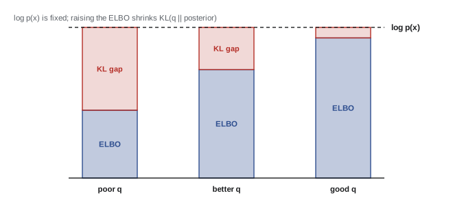
The left side does not depend on \(q\), so minimizing the KL divergence is the same as maximizing the evidence lower bound (ELBO), which involves only the joint distribution \(p(\mathbf x, \mathbf z)\), the model we wrote down. The ELBO has an intuitive split: the first term rewards placing \(q\) where the joint probability is high (fitting the data and prior), and the second, the entropy of \(q\), rewards spreading out. As its name says, the ELBO is also a lower bound on the log evidence, so it can serve as an approximate criterion for model comparison.
The direction of the KL divergence
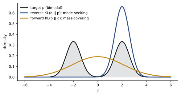
VI minimizes the reverse divergence \(\mathrm{KL}(q\,\|\,p)\), an expectation under \(q\). Where \(q\) puts mass but \(p\) is nearly zero, \(\log(q/p)\) is enormous, so \(q\) is strongly penalized for covering regions the posterior rules out, but barely penalized for missing regions where the posterior has mass. Reverse KL is therefore mode-seeking (or zero-forcing): when the family cannot represent the whole posterior, the optimal \(q\) locks onto one mode and underestimates the spread. The forward divergence \(\mathrm{KL}(p\,\|\,q)\), used by expectation propagation and by maximum likelihood fitting, is mass-covering: it matches moments and spreads \(q\) over all modes, even if that puts mass in the valley between them.
import numpy as np
from scipy.stats import norm
from scipy.optimize import minimize

x = np.linspace(-8, 8, 4001); dx = x[1] - x[0]
p = 0.5 * norm.pdf(x, -2, 0.6) + 0.5 * norm.pdf(x, 2, 0.6)

def kl(a, b):                                  # KL(a || b) on the grid
    mask = a > 1e-300
    return np.sum(a[mask] * (np.log(a[mask]) - np.log(b[mask] + 1e-300))) * dx

def reverse(params):                           # KL(q || p): mode-seeking
    q = norm.pdf(x, params[0], np.exp(params[1]))
    return kl(q, p)

def forward(params):                           # KL(p || q): mass-covering
    q = norm.pdf(x, params[0], np.exp(params[1]))
    return kl(p, q)

for name, obj in [("reverse KL(q||p)", reverse), ("forward KL(p||q)", forward)]:
    for start in [0.5, -1.0]:
        r = minimize(obj, [start, 0.0], method="Nelder-Mead")
print(f"{name}, start mu={start:+.1f}: mu={r.x[0]:+.3f} sd={np.exp(r.x[1]):.3f} KL={r.fun:.3f}")reverse KL(q||p), start mu=+0.5: mu=+1.997 sd=0.605 KL=0.692 reverse KL(q||p), start mu=-1.0: mu=-1.997 sd=0.605 KL=0.692 forward KL(p||q), start mu=+0.5: mu=-0.000 sd=2.088 KL=0.555 forward KL(p||q), start mu=-1.0: mu=-0.000 sd=2.088 KL=0.555
Reverse KL fits a narrow Gaussian to whichever mode is nearer the starting point, ignoring the other entirely; forward KL fits a broad Gaussian centered on the valley, matching the target's mean and variance. Neither is right: the family is simply too poor. In practice, the mode-seeking behavior means that VI answers are sharper than the true posterior, and that VI on a multimodal posterior reports one mode and is confident about it.
Mean-field variational inference
The most common family is the mean-field family, which assumes the latent variables are independent under \(q\): \(q(\mathbf z) = \prod_j q_j(z_j)\). The posterior itself is not assumed to factorize; the approximation simply cannot represent dependence between groups. For this family, the optimal factor \(q_j\) with all the others held fixed has a remarkably general form:
That is, take the log joint, average over all the other factors, and exponentiate. In conjugate-exponential models, which include most of the models of Lessons 1, 3 and 5, this expectation has the same form as the prior, so each factor stays in a standard family and the update reduces to recomputing a few parameters. Cycling through the factors is coordinate ascent variational inference (CAVI); each update increases the ELBO, so CAVI converges, like EM, to a local optimum. EM is in fact the special case in which \(q\) over the latent variables is unrestricted (the exact posterior) and the parameters get point estimates; variational Bayesian EM extends it by also giving the parameters factorized distributions.
A clean example is estimating the mean \(\mu\) and precision \(\tau\) of normal data with the conjugate Normal-Gamma prior. The exact posterior is available, which allows the mean-field answer \(q(\mu)q(\tau)\) to be checked.
import numpy as np
from scipy import stats

rng = np.random.default_rng(4)
x = rng.normal(5.0, 2.0, size=15); N = len(x); xbar = x.mean()
mu0, lam0, a0, b0 = 0.0, 0.1, 1.0, 1.0           # Normal-Gamma prior

# exact posterior (conjugate): tau ~ Gamma(aN, bN), mu | tau ~ N(muN, 1/((lam0+N) tau))
muN = (lam0 * mu0 + N * xbar) / (lam0 + N)
aN = a0 + N / 2
bN = b0 + 0.5 * ((x - xbar) ** 2).sum() + lam0 * N * (xbar - mu0) ** 2 / (2 * (lam0 + N))
mu_marg = stats.t(df=2 * aN, loc=muN, scale=np.sqrt(bN / (aN * (lam0 + N))))

# mean-field CAVI: q(mu) q(tau)
E_tau = 1.0
for it in range(20):
    lamN = (lam0 + N) * E_tau                    # q(mu) = N(muN, 1/lamN)
    E_sq = ((x - muN) ** 2).sum() + N / lamN + lam0 * ((muN - mu0) ** 2 + 1 / lamN)
    a_q = a0 + (N + 1) / 2                       # q(tau) = Gamma(a_q, b_q)
    b_q = b0 + 0.5 * E_sq
    E_tau = a_q / b_q

print(f"posterior mean of mu:   exact {mu_marg.mean():.3f}   CAVI {muN:.3f}")
print(f"posterior sd of mu:     exact {mu_marg.std():.3f}   CAVI {1 / np.sqrt(lamN):.3f}")
print(f"posterior mean of tau:  exact {aN / bN:.4f}  CAVI {E_tau:.4f}")
print(f"implied noise sd: sample {x.std(ddof=1):.3f} 1/sqrt(E[tau]) {1 / np.sqrt(E_tau):.3f}")posterior mean of mu: exact 4.855 CAVI 4.855 posterior sd of mu: exact 0.525 CAVI 0.493 posterior mean of tau: exact 0.2728 CAVI 0.2728 implied noise sd: sample 2.035 1/sqrt(E[tau]) 1.915
CAVI converges in a few iterations. It recovers the posterior means exactly in this model, but its standard deviation for \(\mu\) is about 6% too small, because the true posterior couples \(\mu\) and \(\tau\) (when the noise precision is lower, the mean is less certain), and the factorized \(q\) cannot represent that coupling. This underestimation of uncertainty is the characteristic error of mean-field VI, and it is larger when posterior correlations are stronger.
Worked problem
Mean-field approximation of a correlated Gaussian
The posterior over two parameters is Gaussian with variances 1 and correlation \(\rho\). The mean-field optimum for a Gaussian posterior has each factor's variance equal to the inverse of the corresponding diagonal element of the posterior precision matrix. Find the mean-field standard deviations for \(\rho = 0.5\) and \(\rho = 0.9\).
Show solution
- Covariance \(\Sigma = \begin{pmatrix} 1 & \rho \\ \rho & 1 \end{pmatrix}\); precision \(\Sigma^{-1} = \frac{1}{1 - \rho^2}\begin{pmatrix} 1 & -\rho \\ -\rho & 1 \end{pmatrix}\).
- Mean-field variance: \(1/(\Sigma^{-1})_{11} = 1 - \rho^2\).
- \(\rho = 0.5\): variance 0.75, standard deviation 0.87. \(\rho = 0.9\): variance 0.19, standard deviation 0.44.
Answer: The true marginal standard deviations are 1 in both cases, but mean-field VI reports 0.87 and 0.44. With strong correlation, the approximation is overconfident by more than a factor of two: it matches the width of the posterior across the narrow direction, not along the ridge.
Stochastic and black-box VI
CAVI requires deriving update equations by hand and passes over the whole data set each iteration. Two developments made VI practical for large and non-conjugate models.
Stochastic variational inference
When the log joint is a sum over \(N\) data points, the ELBO's gradient is also a sum, and it can be estimated without bias from a mini-batch, scaled by \(N\) divided by the batch size. Stochastic optimization with decreasing step sizes then converges, exactly as in training neural networks (AI-310). Stochastic VI made topic models and other Bayesian models feasible on millions of documents.
The reparameterization trick
For non-conjugate models, the expectations in the ELBO have no closed form, so they are estimated by Monte Carlo. The difficulty is differentiating an expectation with respect to the parameters of the distribution being sampled. The reparameterization trick writes the random variable as a deterministic, differentiable function of the variational parameters and a fixed noise source. For a Gaussian, \(\mathbf z = \mathbf m + \mathbf s \odot \boldsymbol\epsilon\) with \(\boldsymbol\epsilon \sim \mathcal N(0, I)\), so
which is estimated by averaging gradients over a few noise samples. Combined with automatic differentiation, this gives black-box VI: for any model with a differentiable log joint, the ELBO and its gradient can be computed automatically, and the user only writes the model. The gradient estimates have low variance compared with the alternative score-function (REINFORCE) estimator, which works for discrete variables but is much noisier. Probabilistic programming systems such as Stan (ADVI), PyMC and Pyro offer this automatically.
import numpy as np
rng = np.random.default_rng(0)
n = 60
X = np.column_stack([np.ones(n), rng.normal(size=n), rng.normal(size=n)])
w_true = np.array([-0.5, 1.5, -1.0])
y = (rng.uniform(size=n) < 1 / (1 + np.exp(-X @ w_true))).astype(float)

def grad_logp(W):                         # W: S x 3 samples; prior N(0, 5^2 I)
    p = 1 / (1 + np.exp(-W @ X.T))        # S x n
    return (y - p) @ X - W / 25.0

def logp(w):
    z = X @ w
    return np.sum(y * z - np.logaddexp(0, z)) - w @ w / 50.0

# variational inference: q(w) = N(m, diag(s^2)), reparameterization gradients, Adam
m = np.zeros(3); rho = np.full(3, -1.0)        # s = exp(rho)
state = [np.zeros(3) for _ in range(4)]
lr, b1, b2 = 0.05, 0.9, 0.999
m_avg = np.zeros(3); rho_avg = np.zeros(3)
for t in range(1, 6001):
    lr = 0.05 if t <= 3000 else 0.01
    eps = rng.normal(size=(16, 3))
    s = np.exp(rho)
    W = m + s * eps
    g = grad_logp(W)
    gm = g.mean(axis=0)
    grho = (g * eps * s).mean(axis=0) + 1.0        # +1 from the entropy term
    for i, gr in enumerate([gm, grho]):
        state[2*i] = b1 * state[2*i] + (1 - b1) * gr
        state[2*i+1] = b2 * state[2*i+1] + (1 - b2) * gr ** 2
        step = lr * (state[2*i] / (1 - b1 ** t)) / (np.sqrt(state[2*i+1] / (1 - b2 ** t)) + 1e-8)
        if i == 0: m = m + step
        else: rho = rho + step
    if t > 4000:
        m_avg += m / 2000; rho_avg += rho / 2000
m, s = m_avg, np.exp(rho_avg)

# reference: long random-walk Metropolis run
w = m.copy(); lp = logp(w); samples = []
for it in range(60_000):
    prop = w + 0.35 * rng.normal(size=3)
    lpp = logp(prop)
    if np.log(rng.uniform()) < lpp - lp:
        w, lp = prop, lpp
    if it >= 5000: samples.append(w)
samples = np.array(samples)
C = np.corrcoef(samples.T)
print("            VI mean   MCMC mean    VI sd   MCMC sd")
for j, name in enumerate(["intercept", "w1", "w2"]):
    print(f"{name:10s} {m[j]:8.3f}  {samples[:, j].mean():9.3f}  {s[j]:7.3f}  {samples[:, j].std():8.3f}")
print(f"posterior correlation of w1 and w2 (MCMC): {C[1, 2]:.2f}; mean-field VI assumes 0")VI mean MCMC mean VI sd MCMC sd intercept -0.802 -0.815 0.338 0.370 w1 1.725 1.782 0.459 0.562 w2 -1.142 -1.179 0.364 0.410 posterior correlation of w1 and w2 (MCMC): -0.42; mean-field VI assumes 0
The variational means agree closely with the MCMC reference, but every variational standard deviation is smaller, by up to about 20% for \(w_1\), because the posterior correlations between coefficients are ignored by the mean-field family. A full-covariance Gaussian \(q\) (parameterized by a Cholesky factor) would capture the correlations at the cost of \(O(d^2)\) parameters; normalizing flows go further, transforming a simple distribution through invertible neural networks to represent skewed and multimodal posteriors.
Amortized inference and variational autoencoders
In latent variable models with one latent \(\mathbf z_n\) per data point, classical VI optimizes separate variational parameters for every data point. Amortized inference instead trains an inference network (an encoder) that maps any \(\mathbf x_n\) to the parameters of \(q(\mathbf z_n \mid \mathbf x_n)\), sharing the cost of inference across data points and making inference on new points a single forward pass.
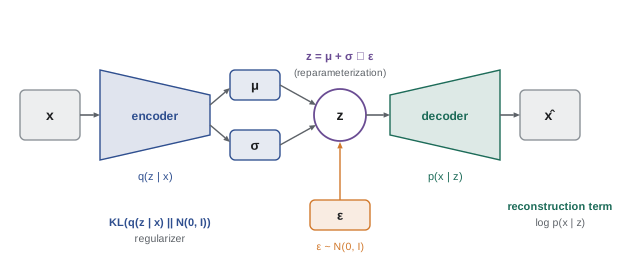
The variational autoencoder (VAE) combines an amortized encoder \(q_\phi(\mathbf z \mid \mathbf x)\) with a neural decoder \(p_\theta(\mathbf x \mid \mathbf z)\) and a simple prior \(p(\mathbf z) = \mathcal N(0, I)\). Both networks are trained together by maximizing the ELBO with reparameterization gradients:
The first term is a reconstruction term, rewarding latent codes from which the decoder can rebuild the input; the second is a regularizer pulling each code distribution toward the prior, which keeps the latent space smooth enough to sample from. New data are generated by drawing \(\mathbf z \sim \mathcal N(0, I)\) and decoding. VAEs are used for representation learning, anomaly detection (inputs with low ELBO are unusual) and, as the compression stage of latent diffusion image generators, inside many modern generative systems.
VI or MCMC?
Neither method dominates; the choice depends on the problem and the purpose:
| Consideration | MCMC | Variational inference |
|---|---|---|
| Accuracy | Asymptotically exact | Biased by the family; typically underestimates variance |
| Speed | Slow; full data each step | Fast; mini-batches, GPUs |
| Scale | Thousands of parameters, moderate data | Millions of parameters and data points |
| Diagnostics | R-hat, ESS, divergences | ELBO convergence; accuracy hard to assess |
| Multimodality | Can mix poorly between modes | Locks onto one mode |
| Typical use | Scientific inference, small to medium models, final answers | Large models, amortized inference, VAEs, quick iteration |
A common workflow uses VI to explore models and initialize, then MCMC for final inference on the chosen model when accurate uncertainty matters, such as in scientific, medical or engineering decisions. For deep learning scale models, approximate methods are the only option: besides VI, the Laplace approximation (a Gaussian at the MAP estimate with covariance from the Hessian), Monte Carlo dropout and deep ensembles are widely used to estimate the uncertainty of neural network predictions. Whatever the method, posterior predictive checks, which simulate data from the fitted model and compare them with the real data, remain the best test of whether the model and its inference make sense.
Lesson 10 shows how to check whether an approximate posterior can be trusted, using simulation-based calibration, and Lesson 12 compares variational methods with ensembles and other ways of capturing uncertainty in deep networks.
Common mistakes
MistakeTrusting mean-field VI uncertainties as calibrated.
InsteadMean-field VI typically underestimates variance, especially with correlated parameters; check against MCMC or use richer families.
MistakeInterpreting a VI fit to a multimodal posterior as complete.
InsteadReverse KL locks onto one mode; run from several initializations or use methods that cover multiple modes.
MistakeComparing models by ELBO as if it were the exact evidence.
InsteadThe ELBO is a lower bound whose gap differs between models; use it cautiously.
MistakeUsing score-function gradients when reparameterization is possible.
InsteadReparameterization gradients have far lower variance for continuous latent variables.
MistakeReporting the last iterate of noisy stochastic VI.
InsteadDecrease the step size and average iterates, and monitor a smoothed ELBO.
Summary and key terms
- VI approximates the posterior by the member of a tractable family closest in KL divergence.
- \(\log p(\mathbf x) = \mathrm{ELBO}(q) + \mathrm{KL}(q\,\|\,p(\mathbf z \mid \mathbf x))\): maximizing the ELBO minimizes the KL without knowing the posterior.
- Reverse KL is mode-seeking and underestimates spread; forward KL is mass-covering.
- Mean-field VI factorizes q; the optimal factor is \(\exp \mathbb E_{-j}[\log p(\mathbf x, \mathbf z)]\), giving CAVI updates in conjugate models.
- Mean-field approximations ignore posterior correlations and are overconfident.
- Stochastic VI uses mini-batch gradients; the reparameterization trick gives low-variance gradients for black-box VI.
- Amortized inference trains an encoder; VAEs maximize a reconstruction term minus a KL regularizer.
- MCMC is asymptotically exact but slow; VI is fast and scalable but biased. Choose by purpose and scale.
- Variational inference
- Approximating a posterior by optimizing over a family of tractable distributions.
- Kullback-Leibler divergence
- An asymmetric measure of how one distribution differs from another.
- ELBO
- Evidence lower bound: the objective maximized by variational inference.
- Mean-field family
- Variational distributions that factorize over variables or groups.
- CAVI
- Coordinate ascent variational inference, updating one factor at a time.
- Mode-seeking
- The tendency of reverse KL to fit one mode of a multimodal target.
- Mass-covering
- The tendency of forward KL to spread over all of the target's mass.
- Stochastic variational inference
- VI using mini-batch estimates of the ELBO gradient.
- Reparameterization trick
- Writing a sample as a differentiable function of parameters and fixed noise.
- Score-function estimator
- A general but high-variance gradient estimator for expectations.
- Amortized inference
- Training a network to output variational parameters for any input.
- Variational autoencoder
- A generative model trained with an amortized encoder and the ELBO.
- Normalizing flow
- An invertible neural transformation used to build flexible distributions.
- Laplace approximation
- A Gaussian approximation at the posterior mode using the Hessian.
Practice problems
Work each problem on paper first, then reveal the answer to check.
Why can VI optimize the ELBO even though the KL divergence to the posterior is unknown?
Show answer
log p(x) = ELBO + KL and log p(x) is constant in q, so maximizing the ELBO minimizes the KL; the ELBO needs only the joint.
Write the ELBO as an expected log joint plus an entropy.
Show answer
ELBO = E_q[log p(x, z)] + H[q], where H[q] = −E_q[log q(z)].
A target has two well-separated modes. Describe the Gaussian fitted by reverse KL and by forward KL.
Show answer
Reverse KL: narrow, on one mode. Forward KL: broad, centered between the modes, matching overall mean and variance.
What is the optimal mean-field factor in general?
Show answer
log q_j*(z_j) = E over the other factors of log p(x, z), plus a constant.
For a Gaussian posterior with unit variances and correlation 0.8, what standard deviation does mean-field VI give?
Show answer
√(1 − 0.64) = 0.6.
A data set has N = 1,000,000 points and mini-batches of 100. How is the mini-batch log-likelihood term scaled in the ELBO gradient?
Show answer
Multiplied by N/B = 10,000.
Write the reparameterization of a Gaussian with mean m and standard deviation s.
Show answer
z = m + s ε with ε ~ N(0, 1).
Why are reparameterization gradients preferred to score-function gradients for continuous latents?
Show answer
They have much lower variance because they use the gradient of the model through the sample.
What are the two terms of a VAE objective and what does each do?
Show answer
Reconstruction log-likelihood (rebuild the input from z) and KL from q(z|x) to the prior (regularize the latent space).
Give one situation favoring MCMC and one favoring VI.
Show answer
MCMC: a medium-sized scientific model needing accurate uncertainty. VI: a large model or data set, or amortized inference in a VAE.
Lesson quiz · 5 questions
Score 60% or more to complete this lesson.
Create a free account to save your progress, take quizzes and earn a certificate.