
AI-320 · Lesson 10 of 12 · 29 min
Probabilistic programming and model checking
The previous lessons derived inference algorithms by hand for particular models. In applied work, analysts rarely do this. They write the model in a probabilistic programming language, and a general-purpose engine (usually Hamiltonian Monte Carlo or variational inference) computes the posterior. That shifts effort from deriving algorithms to the questions that matter more: is the model sensible, did the inference work, does the model reproduce the important features of the data, and which of several models should be trusted? This lesson covers probabilistic programming, the Bayesian workflow, prior and posterior predictive checks, model comparison by cross-validation, sensitivity analysis and the validation of inference itself.
Probabilistic programming languages
A probabilistic program describes how data are generated: draw parameters from priors, compute derived quantities, and draw observations from likelihoods. The language turns this description into a log density and its gradient (by automatic differentiation, AI-310) and hands it to an inference engine. The main systems are:
| System | Host language | Main inference | Notes |
|---|---|---|---|
| Stan | its own language, called from R, Python and others | NUTS (adaptive HMC), variational, optimization | mature diagnostics; widely used in science |
| PyMC | Python | NUTS, variational, SMC | large community; integrates with ArviZ |
| NumPyro | Python (JAX) | NUTS on GPUs, stochastic VI | fast; suits large models |
| Pyro | Python (PyTorch) | stochastic VI, amortized inference | deep generative models |
| Turing.jl | Julia | NUTS, particle methods, Gibbs | flexible composition of samplers |
A hierarchical model of store sales (Lesson 8), for example, takes only a few lines in any of these systems: priors for the population mean \(\mu \sim \mathcal{N}(10, 5^2)\), the spread \(\tau \sim \text{Half-Normal}(0, 3)\) and the noise \(\sigma \sim \text{Half-Normal}(0, 10)\); store effects \(\alpha_j = \mu + \tau z_j\) with \(z_j \sim \mathcal{N}(0, 1)\) (the non-centered form); and observations \(y_{ij} \sim \mathcal{N}(\alpha_j, \sigma^2)\). The engine returns posterior draws of every quantity, from which any summary (means, intervals, the probability that store A beats store B) is computed by averaging over draws.
Most engines need continuous parameters for HMC, so discrete latent variables (mixture assignments, change points) are summed out analytically or handled by samplers that support them. The convenience is real, but a probabilistic programming language does not check that the model makes sense; the workflow does.
The Bayesian workflow
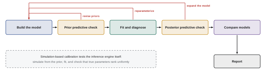
Modern practice treats model building as an iterative cycle rather than a single fit:
- Build: write a model that encodes what is known about how the data arise.
- Check the prior: simulate data from the prior alone and check that it is plausible.
- Fit: run the inference and check its diagnostics (R-hat, effective sample size, divergences, Lesson 7).
- Check the posterior: compare replicated data from the fitted model with the real data.
- Compare and expand: try alternatives, compare predictive performance, and add structure where checks reveal problems.
- Report: summarize with uncertainty, and show how conclusions depend on the choices made.
Prior predictive checks
Priors are hard to judge on the parameter scale, especially when parameters pass through nonlinear links. The prior predictive distribution, the distribution of data implied by the prior alone, puts them on the scale of observations, where domain knowledge is clearer. Draw parameters from the prior, simulate a data set, and look at it.
Worked problem
A "vague" prior that is not vague
A logistic regression has 10 standardized inputs and independent \(\mathcal{N}(0, 10^2)\) priors on each coefficient, chosen to be "uninformative". What does this prior imply about predicted probabilities?
Show solution
- For a typical input vector with entries of size about 1, the linear predictor is a sum of 10 terms each with standard deviation about 10, so its standard deviation is about \(10\sqrt{10} = 32\).
- A linear predictor beyond ±5 gives a probability below 0.007 or above 0.993; with standard deviation 32, about 88% of the prior mass lies there.
Answer: The prior asserts that almost every outcome is nearly certain, a strong and usually absurd claim. A \(\mathcal{N}(0, 1)\) prior (or a scale shrinking with the number of inputs) gives a sensible spread of probabilities. Flat-looking priors on parameters can be highly informative about predictions.
Prior predictive checks also catch errors in model code: simulated sales that are negative, times that run backward, or counts in the billions reveal mistakes before any data are fitted.
Posterior predictive checks
Once the model is fitted, the question is whether it captures the features of the data that matter. The posterior predictive distribution generates replicated data sets \(y^{\text{rep}}\), one per posterior draw, that the model considers plausible. If the observed data look unusual among the replications, the model is missing something.
A test statistic \(T(y)\) chosen to probe a specific feature (the variance, the number of zeros, the largest value, autocorrelation, the proportion of a subgroup) is computed on the observed data and on each replication. The posterior predictive p-value is the fraction of replications with \(T(y^{\text{rep}}) \geq T(y)\); values near 0 or 1 flag misfit. Graphical checks, overlaying histograms or curves of replicated data on the observed data, are often more informative than any single number.
import numpy as np

rng = np.random.default_rng(10)
# Daily defect counts that are really overdispersed (negative binomial, mean 4, r = 1.5)
y = rng.negative_binomial(1.5, 1.5 / (1.5 + 4.0), 60)
n = y.size
print(f"observed: mean {y.mean():.2f}, variance {y.var():.2f}, zeros {np.mean(y == 0):.2f}, max {y.max()}")

# Fit a Poisson model with a Gamma(1, 0.1) prior: the posterior is Gamma(1 + sum y, 0.1 + n)
lam = rng.gamma(1 + y.sum(), 1 / (0.1 + n), 4000)
stats = {"variance/mean": lambda d: d.var() / d.mean(), "fraction of zeros": lambda d: np.mean(d == 0), "maximum": lambda d: d.max()}
rep = rng.poisson(lam[:, None], (lam.size, n))        # one replicated data set per posterior draw
for name, T in stats.items():
    t_obs = T(y)
    t_rep = np.array([T(r) for r in rep])
print(f"{name:18s} observed {t_obs:6.2f}; replicated 95% range {np.percentile(t_rep, 2.5):5.2f} to {np.percentile(t_rep, 97.5):5.2f}; p = {np.mean(t_rep >= t_obs):.3f}")observed: mean 3.77, variance 10.01, zeros 0.08, max 14 variance/mean observed 2.66; replicated 95% range 0.67 to 1.38; p = 0.000 fraction of zeros observed 0.08; replicated 95% range 0.00 to 0.07; p = 0.018 maximum observed 14.00; replicated 95% range 7.00 to 12.00; p = 0.003
Every check fails: the observed variance is 2.7 times the mean, whereas Poisson replications rarely exceed 1.4; the data have more zeros and a larger maximum than the model produces. The Poisson model would give confident but misleading intervals for, say, the probability of a day with more than 10 defects. Note that a good posterior predictive check does not prove a model correct. Checks use the data twice (to fit and to test), so they are conservative, and they only probe the features chosen. They are diagnostics that point toward improvements, not formal tests.
Comparing models by predictive accuracy
When several models survive checking, they can be compared by how well they predict new data. The natural measure is the expected log predictive density (elpd) on new observations, \(\sum_i \log p(y_i^{\text{new}} \mid \mathcal{D})\). Leave-one-out cross-validation estimates it from the data at hand:
Refitting the model \(n\) times is costly, but two approximations use a single set of posterior draws:
- Pareto-smoothed importance sampling (PSIS-LOO) reweights the full-data posterior draws to approximate each leave-one-out posterior, stabilizing the importance weights by fitting a Pareto distribution to their tail. The fitted tail shape \(\hat k\) also diagnoses reliability: values above 0.7 flag observations so influential that the approximation fails, which are often outliers worth examining.
- The widely applicable information criterion (WAIC) is computed from the pointwise log-likelihoods: the log pointwise predictive density minus a penalty equal to the sum over observations of the posterior variance of the log-likelihood. The penalty acts as an effective number of parameters.
import numpy as np
from scipy import stats

rng = np.random.default_rng(10)
y = rng.negative_binomial(1.5, 1.5 / (1.5 + 4.0), 60)

def waic(loglik):                                     # loglik: draws x observations
    lppd = np.sum(np.log(np.mean(np.exp(loglik), axis=0)))
    p_waic = np.sum(np.var(loglik, axis=0))
    return lppd - p_waic, p_waic

# Poisson: conjugate gamma posterior
lam = rng.gamma(1 + y.sum(), 1 / (0.1 + y.size), 4000)
ll_pois = stats.poisson.logpmf(y[None, :], lam[:, None])

# Negative binomial: posterior on a grid over (mean, r) with flat priors, then sampled
mus = np.linspace(2, 8, 121); rs = np.linspace(0.3, 6, 115)
M, R = np.meshgrid(mus, rs, indexing="ij")
logpost = np.array([[stats.nbinom.logpmf(y, r, r / (r + m)).sum() for r in rs] for m in mus])
w = np.exp(logpost - logpost.max()).ravel(); w /= w.sum()
idx = rng.choice(w.size, 4000, p=w)
m_s, r_s = M.ravel()[idx], R.ravel()[idx]
ll_nb = stats.nbinom.logpmf(y[None, :], r_s[:, None], (r_s / (r_s + m_s))[:, None])

for name, ll in (("Poisson", ll_pois), ("negative binomial", ll_nb)):
    elpd, p = waic(ll)
    print(f"{name:18s} elpd_WAIC {elpd:8.1f}   effective parameters {p:4.1f}")
print(f"posterior mean of r for the negative binomial: {r_s.mean():.2f} (true 1.5)")Poisson elpd_WAIC -163.0 effective parameters 2.6 negative binomial elpd_WAIC -144.6 effective parameters 1.9 posterior mean of r for the negative binomial: 2.67 (true 1.5)
The negative binomial is better by about 18 units of elpd, a decisive difference (differences are judged against their standard error, computed from the pointwise values; a difference of a few units with a similar standard error is not meaningful). A telling detail: the Poisson model has one parameter but an effective number of 2.6, a symptom of misspecification, since a well-specified model's penalty is close to its parameter count. The dispersion parameter \(r\) is only loosely determined by 60 observations, as its posterior mean of 2.7 against the true 1.5 shows.
Predictive comparison differs from the Bayes factors of Lesson 1. Bayes factors compare marginal likelihoods, which depend strongly on the prior width even when the posterior does not, and answer the question of which model is more probable if one of them is true. Cross-validation asks which model predicts better, a question that remains meaningful when all models are approximations. Instead of selecting one model, predictions can also be combined: stacking finds the weights for a mixture of models that maximize the leave-one-out predictive density.
Sensitivity analysis and reporting
Every model rests on choices: priors, likelihoods, which data to include, how to handle outliers. A sensitivity analysis refits with reasonable alternatives and reports how much the conclusions change. If the conclusion survives, it is robust; if it hinges on one choice, readers need to know. Power-scaling methods estimate prior and likelihood sensitivity cheaply by reweighting the existing draws.
Good reporting of a Bayesian analysis includes: the model in full (priors and likelihood); the inference method and its diagnostics; posterior summaries with intervals rather than point estimates alone; the results of predictive checks; and any sensitivity analysis. Posterior probabilities of practically meaningful statements ("the probability that the new process reduces defects by at least 10% is 0.87") communicate more to decision-makers than coefficient tables.
Validating the inference itself
Diagnostics such as R-hat detect many sampling failures, but not all, and custom samplers or variational approximations can be subtly wrong. Simulation-based calibration (SBC) tests the inference machinery: draw parameters \(\tilde\theta\) from the prior, simulate data from them, run the inference, and record the rank of \(\tilde\theta\) among the posterior draws. If the inference is correct, the ranks are uniformly distributed over many repetitions, because the true parameter is then just another draw from the posterior. Histograms of the ranks that are U-shaped indicate posteriors that are too narrow; humps indicate posteriors that are too wide; slopes indicate bias.
Worked problem
Reading an SBC histogram
An SBC run with 500 simulations and 99 posterior draws each shows that the true parameter falls below all 99 draws in 60 simulations and above all of them in 55, far more than expected. What does this say?
Show solution
- With correct inference, each of the 100 possible ranks has probability 0.01, so about 5 simulations should land in each extreme bin.
- Instead, 115 of 500 land in the two extremes: the posterior often fails to cover the truth at all.
Answer: The posteriors are much too narrow: the inference understates uncertainty, as mean-field variational inference often does (Lesson 9). The remedy is a richer approximation or MCMC.
Common mistakes
MistakeAssuming wide priors on parameters are uninformative.
InsteadRun prior predictive checks; wide priors can imply extreme predictions.
MistakeReporting a posterior without checking that the model reproduces the data.
InsteadUse posterior predictive checks with statistics that probe important features.
MistakeTreating a passed predictive check as proof of a correct model.
InsteadChecks only test the features chosen and use the data twice.
MistakeDeclaring a winner from a small elpd difference.
InsteadCompare the difference with its standard error and check Pareto \(\hat k\) values.
MistakeTrusting new inference code because it runs without errors.
InsteadValidate it with simulation-based calibration.
Summary and key terms
- Probabilistic programming languages turn a generative description into a posterior using general engines such as NUTS and variational inference.
- The Bayesian workflow cycles through building, checking, fitting, comparing and reporting.
- Prior predictive checks reveal implausible priors and coding errors on the scale of data.
- Posterior predictive checks compare replicated and observed data to expose misfit.
- PSIS-LOO and WAIC estimate predictive accuracy from posterior draws; stacking combines models.
- Sensitivity analysis and simulation-based calibration test the robustness of conclusions and the correctness of inference.
- Probabilistic programming language
- A language for writing generative models whose posteriors are computed automatically.
- Prior predictive distribution
- The distribution of data implied by the prior alone.
- Posterior predictive check
- Comparing replicated data from the fitted model with the observed data.
- Posterior predictive p-value
- The fraction of replications whose test statistic exceeds the observed one.
- elpd
- Expected log predictive density for new data.
- PSIS-LOO
- Leave-one-out cross-validation approximated by Pareto-smoothed importance sampling.
- WAIC
- An information criterion based on pointwise log-likelihood means and variances.
- Stacking
- Weighting models to maximize the leave-one-out predictive density of their mixture.
- Sensitivity analysis
- Refitting under alternative assumptions to see how conclusions change.
- Simulation-based calibration
- Testing inference by checking that ranks of true parameters among posterior draws are uniform.
Practice problems
Work each problem on paper first, then reveal the answer to check.
Name the five main stages of the Bayesian workflow.
Show answer
Build, prior check, fit and diagnose, posterior check, compare and report.
A logistic model with 4 standardized inputs has \(\mathcal{N}(0, 5^2)\) priors. Rough prior standard deviation of the linear predictor?
Show answer
\(5\sqrt4 = 10\).
What test statistic would check whether a Poisson model handles excess zeros?
Show answer
The fraction of zeros.
A posterior predictive p-value of 0.48 for the variance means:
Show answer
The model reproduces the variance well.
Why are posterior predictive checks conservative?
Show answer
The data are used both to fit and to test.
What does a Pareto \(\hat k\) above 0.7 indicate?
Show answer
An influential observation for which PSIS-LOO is unreliable.
WAIC effective parameters much larger than the real number suggests:
Show answer
Misspecification or highly influential observations.
Model A beats model B by 2.1 elpd with standard error 2.5. Conclusion?
Show answer
No clear difference.
What do U-shaped SBC rank histograms indicate?
Show answer
Posteriors that are too narrow.
How does stacking differ from choosing the best model?
Show answer
It combines models with weights that maximize predictive performance.
Lesson quiz · 5 questions
Score 60% or more to complete this lesson.
Create a free account to save your progress, take quizzes and earn a certificate.