Learning graphical models, loopy inference and causality

Lesson 3 took the graph and its conditional distributions as given and asked how to compute probabilities from them. In practice both usually come from data. This lesson covers learning the parameters of a graphical model, learning its structure, approximate inference in graphs with loops where exact methods are too expensive, conditional random fields for labeling sequences and images, and causal graphical models, which answer a different kind of question: not what we expect to see if we observe something, but what would happen if we intervened to change it.

Learning parameters from complete data

Suppose the structure of a Bayesian network is known and every variable is observed in every training case. The log-likelihood of the data then splits into a separate term for each node:

Each node's parameters \(\boldsymbol\theta_j\) appear in only one term, so they can be estimated independently. This decomposability is one of the great practical strengths of Bayesian networks. For discrete variables, the maximum likelihood estimate of each conditional probability table entry is a ratio of counts:

Rare parent configurations give unreliable or undefined ratios (zero divided by zero, or a probability of exactly zero for an outcome merely not yet seen). The standard remedy is a Dirichlet prior on each row of the table (Lesson 1), which adds pseudo-counts \(\alpha\) to every cell: \(\hat p = (N_{kc} + \alpha)/(N_c + K\alpha)\). With \(\alpha = 1\) this is Laplace or add-one smoothing.

For continuous nodes, each conditional is a regression: a linear Gaussian node \(x_j \mid \mathrm{pa} \sim \mathcal{N}(\mathbf{w}^\top\mathrm{pa} + b, \sigma^2)\) is fitted by least squares. When some variables are missing in some cases, or are never observed (latent variables), the likelihood no longer decomposes, and the EM algorithm of Lesson 5 is the standard tool: it fills in expected counts using inference and then re-estimates the tables as if the data were complete.

Learning structure

Learning which edges exist is harder. The number of possible DAGs grows super-exponentially (25 for three nodes, 29,000 for five, more than \(10^{18}\) for ten), so structure learning needs both a criterion and a search strategy. There are two broad approaches.

Score-based methods assign each candidate structure a score that rewards fit and penalizes complexity, then search for a high-scoring structure. The likelihood alone always favors adding edges, because a more flexible model never fits worse, so a penalty is essential. The Bayesian information criterion (BIC) approximates the log marginal likelihood (Lesson 1):

where \(k\) is the number of free parameters. Because the score decomposes over nodes, local search is efficient: start from an empty or guessed graph and repeatedly add, delete or reverse the single edge that most improves the score, keeping the graph acyclic, until no change helps. Restarts or tabu lists help escape local optima.

import numpy as np

rng = np.random.default_rng(11)
n = 2000
# True structure: smoking (S) -> tar (T) -> cancer (C); S has no direct edge to C
S = rng.random(n) < 0.3
T = rng.random(n) < np.where(S, 0.8, 0.1)
C = rng.random(n) < np.where(T, 0.25, 0.03)

def loglik_cpt(child, parents):
    """Maximum likelihood log-likelihood of a binary child given binary parents, with counts."""
    ll, k = 0.0, 0
    keys = np.zeros(n, dtype=int)
    for p in parents:
        keys = keys * 2 + p
    for key in np.unique(keys):
        m = keys == key
        c1, c0 = child[m].sum(), (~child[m]).sum()
        for c in (c1, c0):
            if c > 0:
                ll += c * np.log(c / (c1 + c0))
        k += 1                                        # one free parameter per parent configuration
    return ll, k

def bic(structure):
    total_ll, total_k = 0.0, 0
    for child, parents in structure:
        ll, k = loglik_cpt(child, parents)
        total_ll += ll; total_k += k
    return total_ll - 0.5 * total_k * np.log(n), total_ll, total_k

candidates = {
    "S -> T -> C (true)": [(S, []), (T, [S]), (C, [T])],
    "S -> T -> C plus S -> C": [(S, []), (T, [S]), (C, [T, S])],
    "S -> C, no tar edge": [(S, []), (T, []), (C, [S])],
    "all independent": [(S, []), (T, []), (C, [])],
}
for name, st in candidates.items():
    b, ll, k = bic(st)
    print(f"{name:26s} log-lik {ll:9.1f}  params {k}  BIC {b:9.1f}")

# Learned conditional probability table with add-one (Dirichlet) smoothing
for t in (True, False):
    m = T == t
    print(f"P(C | T={int(t)}) = {(C[m].sum() + 1) / (m.sum() + 2):.3f}  from {m.sum()} cases")

S -> T -> C (true)         log-lik   -2542.8  params 5  BIC   -2561.8
S -> T -> C plus S -> C    log-lik   -2542.4  params 7  BIC   -2569.0
S -> C, no tar edge        log-lik   -3088.5  params 4  BIC   -3103.7
all independent            log-lik   -3138.0  params 3  BIC   -3149.4
P(C | T=1) = 0.248  from 636 cases
P(C | T=0) = 0.030  from 1364 cases

The extra edge from smoking to cancer improves the log-likelihood by less than one unit but costs two parameters, so BIC rejects it, correctly, because in this simulation smoking acts only through tar. Removing the tar edge destroys the fit. The learned conditional probabilities are close to the true 0.25 and 0.03.

Constraint-based methods instead test conditional independences in the data and build a graph consistent with them. The PC algorithm starts with a complete undirected graph, removes the edge between two variables whenever some set of other variables makes them conditionally independent, and then orients edges using v-structures (colliders, Lesson 3): if A and C are both adjacent to B but not to each other, and B was not in the set that separated them, the pattern must be A → B ← C.

Both approaches face a fundamental limit. Different DAGs can encode exactly the same conditional independences; A → B → C, A ← B ← C and A ← B → C are all equivalent. Such Markov-equivalent graphs fit any observational data equally well, so data alone can identify only an equivalence class, in which some edge directions remain undetermined. Fixing them requires background knowledge (time order, physics) or experiments, which leads to the causal questions at the end of this lesson.

Inference in graphs with loops

Variable elimination and message passing are exact and efficient on chains and trees (Lesson 3). On graphs with loops, exact inference is possible with the junction tree algorithm, which clusters variables into a tree of cliques and passes messages between the clusters. Its cost is exponential in the size of the largest cluster, measured by the graph's treewidth. For a grid of pixels, the treewidth equals the shorter side of the grid, so exact inference on even a 100 × 100 image would require tables of \(2^{100}\) entries. Exact inference in general graphical models is NP-hard, and approximation is unavoidable.

Loopy belief propagation simply runs the sum-product message updates on the loopy graph anyway, iterating until the messages stop changing. Each node combines the messages from its neighbors with its own evidence to form a belief, and sends each neighbor a message based on everything except what that neighbor told it. There is no guarantee of convergence or correctness, because messages can circulate around loops and count the same evidence repeatedly, but in many problems it works remarkably well. The decoding of turbo codes and LDPC codes, used in every mobile phone and Wi-Fi connection, is loopy belief propagation.

A classic test is image denoising with an Ising model. Each pixel \(x_i \in \{-1, +1\}\) is linked to its four neighbors with a coupling that rewards agreement, and to its noisy observation \(y_i\):

For binary variables, messages can be represented as single numbers (log-odds), and the sum-product update takes the compact form \(m_{j \to i} = \tanh^{-1}\!\left(\tanh J \tanh\left(h y_j + \sum_{k \neq i} m_{k \to j}\right)\right)\).

import numpy as np

rng = np.random.default_rng(1)
H, W = 40, 40
yy, xx = np.mgrid[0:H, 0:W]
clean = np.where((xx - 20) ** 2 + (yy - 20) ** 2 < 120, 1, -1)       # a disc of +1 on a -1 background
flip = rng.random((H, W)) < 0.2
noisy = np.where(flip, -clean, clean)

J, h = 0.9, 0.7      # coupling between neighbours and strength of the evidence (Ising model)
# messages m[d][i, j] = message into pixel (i, j) from its neighbour in direction d, as a log-odds
msgs = {d: np.zeros((H, W)) for d in "udlr"}
def shift(a, d):
    out = np.zeros_like(a)
    if d == "u": out[1:, :] = a[:-1, :]          # value of the pixel above
    if d == "d": out[:-1, :] = a[1:, :]
    if d == "l": out[:, 1:] = a[:, :-1]
    if d == "r": out[:, :-1] = a[:, 1:]
    return out
opposite = {"u": "d", "d": "u", "l": "r", "r": "l"}
for it in range(15):
    belief = h * noisy + sum(msgs.values())
    new = {}
    for d in "udlr":
        # the neighbour in direction d sends what it believes, excluding what this pixel told it
        nb_belief = shift(belief, d)
        nb_from_me = shift(msgs[opposite[d]], d)
        x = nb_belief - nb_from_me
        new[d] = np.arctanh(np.tanh(J) * np.tanh(x))
        if d == "u": new[d][0, :] = 0
        if d == "d": new[d][-1, :] = 0
        if d == "l": new[d][:, 0] = 0
        if d == "r": new[d][:, -1] = 0
    msgs = new
    if it in (0, 2, 14):
        est = np.where(h * noisy + sum(msgs.values()) > 0, 1, -1)
        print(f"iteration {it + 1:2d}: pixel error {np.mean(est != clean):.3f}")
print(f"noisy image pixel error {np.mean(noisy != clean):.3f}")

iteration  1: pixel error 0.075
iteration  3: pixel error 0.011
iteration 15: pixel error 0.006
noisy image pixel error 0.190

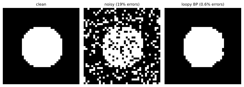
The neighbors' agreement outweighs isolated wrong observations, while pixels along the true boundary, where neighbors genuinely disagree, are where the remaining errors sit. When loopy belief propagation fails to converge, damping (averaging each new message with the old one) usually helps. The alternatives are sampling methods (Gibbs sampling, Lesson 7) and variational methods (Lesson 9); loopy belief propagation can itself be understood as minimizing an approximate free energy, linking it to variational inference.

Conditional random fields

Generative models such as HMMs and naive Bayes model the joint distribution \(p(\mathbf{x}, \mathbf{y})\) of inputs and labels. When the goal is only to predict labels from inputs, it is often better to model \(p(\mathbf{y} \mid \mathbf{x})\) directly, which frees the model from describing how inputs are generated and allows rich, overlapping input features. A conditional random field (CRF) is an undirected graphical model over the labels, conditioned on the input:

In a linear-chain CRF for sequence labeling (part-of-speech tags, named entities, or segments of a sensor signal), the features \(\mathbf{f}\) can look at any part of the input (the current word, its suffix, whether it is capitalized, the next word) together with adjacent label pairs. Inference uses the same forward-backward and Viterbi algorithms as an HMM, because the label graph is still a chain. Training maximizes the conditional log-likelihood, which is concave in \(\mathbf{w}\); its gradient is the observed feature counts minus the expected counts under the model, computed by forward-backward.

A CRF relates to an HMM as logistic regression relates to naive Bayes: the discriminative partner of a generative model. Today, neural sequence models often compute the input features, with a CRF layer on top to enforce consistent label sequences (for example, that an "inside a name" tag cannot follow an "outside" tag). Grid-shaped CRFs serve the same role in image segmentation, encouraging neighboring pixels to take the same label unless the image shows an edge.

Causal graphical models

A Bayesian network describes how variables are associated. A causal graphical model makes a stronger claim: each edge represents a direct causal influence, so the graph also predicts what happens under interventions. The distinction is captured by the do-operator. \(p(y \mid x)\) is the distribution of \(Y\) among cases where \(X\) happened to equal \(x\); \(p(y \mid \mathrm{do}(x))\) is the distribution of \(Y\) if we set \(X\) to \(x\) by intervention. In the graph, an intervention deletes all arrows into \(X\), because its value is no longer determined by its usual causes.

The two differ when a confounder affects both \(X\) and \(Y\). A standard example: doctors give a treatment more often to severely ill patients, and severe illness lowers recovery. Treated patients may then recover no more often than untreated ones, even though the treatment helps, because the treated group is sicker. This is Simpson's paradox: an association that reverses or disappears when data are split by a third variable.

If the confounders \(Z\) are observed and satisfy the back-door criterion (they block every path from \(X\) to \(Y\) that starts with an arrow into \(X\), and contain no descendant of \(X\)), the causal effect can be computed from observational data by adjustment:

Compare this with ordinary conditioning, \(p(y \mid x) = \sum_z p(y \mid x, z)\,p(z \mid x)\): the adjustment weights each stratum by how common it is overall, not by how common it is among the treated.

import numpy as np

rng = np.random.default_rng(5)
n = 200000
# Severity Z confounds treatment X and recovery Y: severe patients get treated more and recover less
Z = rng.random(n) < 0.4
X = rng.random(n) < np.where(Z, 0.8, 0.2)
Y = rng.random(n) < 0.5 + 0.2 * X - 0.35 * Z          # treatment truly adds 0.20 to recovery

obs = Y[X].mean() - Y[~X].mean()
print(f"observational difference P(Y|X=1) - P(Y|X=0): {obs:+.3f}")

# Back-door adjustment: average the within-stratum effect over the distribution of Z
adj = 0.0
for z in (True, False):
    m = Z == z
    effect = Y[m & X].mean() - Y[m & ~X].mean()
    adj += effect * m.mean()
    print(f"  within Z={int(z)}: treated {Y[m & X].mean():.3f}, untreated {Y[m & ~X].mean():.3f}")
print(f"adjusted estimate of P(Y|do(X=1)) - P(Y|do(X=0)): {adj:+.3f}")

# A randomized experiment cuts the arrow Z -> X
Xr = rng.random(n) < 0.5
Yr = rng.random(n) < 0.5 + 0.2 * Xr - 0.35 * Z
print(f"randomized experiment difference: {Yr[Xr].mean() - Yr[~Xr].mean():+.3f}")

observational difference P(Y|X=1) - P(Y|X=0): -0.009
  within Z=1: treated 0.345, untreated 0.149
  within Z=0: treated 0.703, untreated 0.501
adjusted estimate of P(Y|do(X=1)) - P(Y|do(X=0)): +0.199
randomized experiment difference: +0.203

Randomization works because assigning treatment by coin flip deletes the arrow from severity to treatment, exactly what the do-operator describes. When randomization is impossible, adjustment is only as good as the assumption that every confounder has been measured, and that assumption cannot be tested from the data. Adjusting for the wrong variables can also create bias: conditioning on a collider (a common effect) or on a mediator (a step on the causal path) distorts the estimate. Drawing the causal graph forces these assumptions into the open.

Causal reasoning matters wherever models inform decisions. A model predicting hospital readmission from treatment records learns associations, including confounded ones; using it to decide who should receive a treatment asks a causal question it was never built to answer. Uplift modeling in marketing, policy evaluation, and fairness analysis all require causal rather than merely predictive models.