
AI-320 · Lesson 12 of 12 · 31 min
Uncertainty in machine learning and a capstone project
The course has built a toolkit for reasoning under uncertainty: Bayesian updating, exponential families, graphical models, latent variables, Gaussian processes, Monte Carlo, Bayesian regression, variational inference, model checking and state-space models. This final lesson turns to how these ideas are used with modern machine learning systems, whose predictions drive decisions in medicine, finance, engineering and autonomous systems. It covers the kinds of uncertainty a model faces, calibration, practical methods for uncertainty in deep networks, conformal prediction, Bayesian optimization, and a capstone project that combines the course's methods into a decision-making system.
Two kinds of uncertainty
It helps to separate two sources of uncertainty in a prediction:
- Aleatoric uncertainty is the randomness inherent in the outcome given the inputs: the noise in a sensor, the unpredictable part of a customer's choice. More data of the same kind does not reduce it. It is captured by the likelihood, for example the noise variance \(\sigma^2\) in regression.
- Epistemic uncertainty is uncertainty about the model itself, arising from limited data. It is large for inputs unlike the training data and shrinks as data accumulate. It is captured by the posterior over parameters or functions.
The predictive variance of Bayesian linear regression (Lesson 8) shows both: \(\sigma^2\) is aleatoric and \(\boldsymbol\phi_*^\top\mathbf{S}\boldsymbol\phi_*\) is epistemic. The distinction guides action: high epistemic uncertainty suggests collecting more data in that region or deferring to a human; high aleatoric uncertainty suggests that better inputs, not more examples, are needed.
Worked problem
Splitting predictive uncertainty
A model predicting delivery time has noise variance 4 min², and the posterior parameter variance contributes 0.5 min² for a typical urban order but 12 min² for an order to a new rural area. Compare the predictive standard deviations and what each case needs.
Show solution
- Urban: \(\sqrt{4 + 0.5} = 2.1\) minutes, almost all aleatoric.
- Rural: \(\sqrt{4 + 12} = 4.0\) minutes, mostly epistemic.
Answer: Urban predictions are as good as the inputs allow; improving them needs new inputs (traffic, weather). Rural predictions would improve with more rural deliveries, so the right response is to collect data there and quote wider windows meanwhile.
Calibration
A model is calibrated if its stated probabilities match observed frequencies: among all cases where it says 80%, about 80% should turn out positive. Calibration is separate from accuracy; a model can rank cases well yet be badly overconfident. Modern deep networks trained to minimize cross-entropy are often overconfident, especially large ones trained for many epochs.
Calibration is measured with a reliability diagram, which bins predictions by confidence and plots observed accuracy against mean confidence in each bin, and summarized by the expected calibration error (ECE), the bin-weighted average gap. Proper scoring rules, which are optimized only by the true probabilities, assess calibration and sharpness together: the log loss (negative log-likelihood) and the Brier score (mean squared error of the probabilities).
The simplest repair is temperature scaling: divide the network's logits by a single learned temperature \(T > 1\) before the softmax, choosing \(T\) to minimize the negative log-likelihood on held-out validation data. Because dividing all logits by the same number does not change their order, accuracy is unchanged.
import numpy as np

rng = np.random.default_rng(14)
n, k = 6000, 5
true_logits = rng.normal(0, 1.5, (n, k))
probs_true = np.exp(true_logits) / np.exp(true_logits).sum(1, keepdims=True)
y = np.array([rng.choice(k, p=p) for p in probs_true])
model_logits = 2.5 * true_logits                      # an overconfident model: right ranking, too sharp

def softmax(z):
    z = z - z.max(1, keepdims=True); e = np.exp(z); return e / e.sum(1, keepdims=True)

def ece(p, y, bins=10):
    conf, pred = p.max(1), p.argmax(1)
    total = 0.0
    for lo in np.linspace(0, 1, bins, endpoint=False):
        m = (conf > lo) & (conf <= lo + 1 / bins)
        if m.any():
            total += m.mean() * abs(np.mean(pred[m] == y[m]) - conf[m].mean())
    return total

val, test = slice(0, 3000), slice(3000, n)
nll = lambda T, s: -np.mean(np.log(softmax(model_logits[s] / T)[np.arange(s.stop - s.start), y[s]]))
Ts = np.linspace(0.5, 5, 451)
T_best = Ts[np.argmin([nll(T, val) for T in Ts])]     # fit one temperature on validation data
for name, T in (("before scaling", 1.0), (f"temperature {T_best:.2f}", T_best)):
    p = softmax(model_logits[test] / T)
print(f"{name:18s} accuracy {np.mean(p.argmax(1) == y[test]):.3f} mean confidence {p.max(1).mean():.3f} ECE {ece(p, y[test]):.3f} NLL {nll(T, test):.3f}")before scaling accuracy 0.578 mean confidence 0.788 ECE 0.211 NLL 1.431 temperature 2.55 accuracy 0.578 mean confidence 0.558 ECE 0.026 NLL 1.083
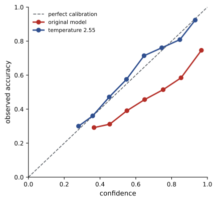
The model's mean confidence of 0.79 against an accuracy of 0.58 is the overconfidence typical of large networks. One parameter, fitted on validation data, removes almost all of the calibration error and improves the log loss substantially, without changing a single prediction. More flexible methods (Platt scaling with a full linear map, isotonic regression, histogram binning) handle more complex miscalibration but need more validation data. Calibration must be checked again after any shift in the data, because a model calibrated on one population is rarely calibrated on another.
Uncertainty in deep networks
Full Bayesian inference over the millions or billions of weights in a deep network is impractical, but several approximations capture useful epistemic uncertainty:
| Method | Idea | Cost | Notes |
|---|---|---|---|
| Deep ensembles | train several networks from different random initializations and average their predictions | several times training and inference | strong and simple; disagreement signals epistemic uncertainty |
| Monte Carlo dropout | keep dropout on at test time and average many stochastic forward passes | many forward passes | cheap to add; a crude variational approximation |
| Laplace approximation | fit a Gaussian at the trained weights using the curvature (often only for the last layer) | one Hessian approximation | post hoc; no retraining |
| SWAG | fit a Gaussian to the weights visited by SGD late in training | small extra training cost | captures the local shape of the loss surface |
| Variational Bayes | learn a distribution over weights by maximizing the ELBO (Lesson 9) | roughly twice the parameters | principled but often underfits at scale |
Deep ensembles are usually the strongest baseline: networks trained from different starting points end up in different modes of the loss surface, so their disagreement reflects genuine uncertainty about the function. They can be seen as a coarse sample from the posterior. A last-layer Laplace approximation is attractive when retraining is impossible, as with a large pre-trained model. Whatever the method, uncertainty estimates should be evaluated: by calibration on held-out data, by how well uncertainty detects out-of-distribution inputs, and by whether rejecting the most uncertain predictions improves accuracy on the rest.
Large language models raise the same questions. Their token probabilities are reasonably calibrated after pre-training but often less so after fine-tuning for instruction following, and confidence expressed in words may not match the underlying probabilities. Sampling several answers and measuring their agreement (self-consistency) is a practical ensemble-like signal.
Conformal prediction
Bayesian uncertainty is only as reliable as the model and the prior. Conformal prediction offers a guarantee that does not depend on the model being correct. Given any trained predictor and a held-out calibration set, split conformal prediction computes a score for each calibration example measuring how badly the model did, such as the absolute residual \(|y_i - \hat y(x_i)|\), and takes the \(\lceil(n + 1)(1 - \alpha)\rceil\)-th smallest score as \(\hat q\). The prediction interval for a new input is \(\hat y(x) \pm \hat q\). If calibration and test examples are exchangeable (for example, independent draws from the same distribution), the interval contains the true value with probability at least \(1 - \alpha\), whatever the model and whatever the data distribution.
import numpy as np

rng = np.random.default_rng(15)
def make(n):
    x = rng.uniform(0, 10, n)
    y = np.sin(x) * 3 + rng.normal(0, 0.3 + 0.15 * x, n)      # noise grows with x
    return x, y
xtr, ytr = make(500); xcal, ycal = make(500); xte, yte = make(5000)

coef = np.polyfit(xtr, ytr, 7)                         # any point predictor will do
pred = lambda x: np.polyval(coef, x)

alpha = 0.1                                            # target 90% coverage
scores = np.abs(ycal - pred(xcal))                     # conformity scores on held-out calibration data
nq = int(np.ceil((len(scores) + 1) * (1 - alpha)))
qhat = np.sort(scores)[nq - 1]
covered = np.abs(yte - pred(xte)) <= qhat
print(f"interval half-width {qhat:.2f}; test coverage {covered.mean():.3f} (target 0.90)")
for lo, hi in ((0, 3), (3, 7), (7, 10)):
    m = (xte >= lo) & (xte < hi)
print(f" x in [{lo}, {hi}): coverage {covered[m].mean():.3f}")interval half-width 1.96; test coverage 0.902 (target 0.90) x in [0, 3): coverage 1.000 x in [3, 7): coverage 0.920 x in [7, 10): coverage 0.784
The guarantee holds on average over all inputs (marginal coverage), not for each input separately. Here, with noise growing with \(x\), a constant-width interval over-covers where the noise is small and under-covers where it is large. Better scores fix this: conformalized quantile regression uses predicted quantiles as the base intervals and adjusts them, giving intervals that widen where the data are noisy. For classification, conformal methods return prediction sets, which contain several labels when the model is unsure. The exchangeability assumption is the weak point: under distribution shift the guarantee can fail, and weighted or adaptive variants are needed.
Bayesian optimization
Many problems require optimizing a function that is expensive to evaluate and gives no gradients: tuning the hyperparameters of a model that takes hours to train, choosing process settings in a chemical plant, designing a material or an antenna through simulation. Bayesian optimization builds a probabilistic surrogate of the function, usually a Gaussian process (Lesson 6), from the evaluations so far, and uses it to decide where to evaluate next. An acquisition function scores each candidate by balancing exploitation (where the surrogate predicts good values) and exploration (where it is uncertain):
- Expected improvement (EI): the expected amount by which a candidate beats the best value so far, which has a closed form under a Gaussian predictive distribution: \(\mathrm{EI}(x) = (f^* - \mu)\Phi(z) + \sigma\varphi(z)\) with \(z = (f^* - \mu)/\sigma\) for minimization.
- Upper (or lower) confidence bound: \(\mu(x) \pm \kappa\sigma(x)\), with \(\kappa\) setting the exploration level.
- Thompson sampling: draw one function from the posterior and evaluate at its optimum.
import numpy as np
from scipy.stats import norm

rng = np.random.default_rng(16)
f = lambda x: -(np.sin(3 * x) + 0.5 * np.cos(7 * x) + 0.2 * x)    # expensive black box to minimize
grid = np.linspace(0, 3, 601)

def gp(Xo, yo, Xs, ell=0.3, sn=1e-3):
    k = lambda a, b: np.exp(-0.5 * (a[:, None] - b[None, :]) ** 2 / ell ** 2)
    mu0, sd0 = yo.mean(), yo.std() + 1e-9
    yn = (yo - mu0) / sd0
    L = np.linalg.cholesky(k(Xo, Xo) + sn * np.eye(len(Xo)))
    a = np.linalg.solve(L.T, np.linalg.solve(L, yn))
    Ks = k(Xs, Xo); v = np.linalg.solve(L, Ks.T)
    var = np.clip(1 - np.sum(v ** 2, 0), 1e-12, None)
    return mu0 + sd0 * (Ks @ a), sd0 * np.sqrt(var)

X = rng.uniform(0, 3, 3); y = f(X)
for it in range(10):
    mu, sd = gp(X, y, grid)
    best = y.min()
    z = (best - mu) / sd
    ei = (best - mu) * norm.cdf(z) + sd * norm.pdf(z)          # expected improvement
    x_next = grid[np.argmax(ei)]
    X = np.append(X, x_next); y = np.append(y, f(x_next))
    print(f"evaluation {it + 4:2d}: x = {x_next:.3f}, f = {f(x_next):+.3f}, best so far {y.min():+.3f}")
print(f"true minimum on the grid: {f(grid).min():+.3f} at x = {grid[np.argmin(f(grid))]:.3f}")
print(f"random search with 13 evaluations, average best: {np.mean([f(rng.uniform(0, 3, 13)).min() for _ in range(2000)]):+.3f}")evaluation 4: x = 0.055, f = -0.639, best so far -0.639 evaluation 5: x = 2.335, f = -0.726, best so far -0.726 evaluation 6: x = 2.625, f = -1.970, best so far -1.970 evaluation 7: x = 2.795, f = -1.799, best so far -1.970 evaluation 8: x = 2.675, f = -2.017, best so far -2.017 evaluation 9: x = 0.725, f = -1.145, best so far -2.017 evaluation 10: x = 2.680, f = -2.017, best so far -2.017 evaluation 11: x = 2.675, f = -2.017, best so far -2.017 evaluation 12: x = 2.675, f = -2.017, best so far -2.017 evaluation 13: x = 2.675, f = -2.017, best so far -2.017 true minimum on the grid: -2.017 at x = 2.680 random search with 13 evaluations, average best: -1.784
After exploring both ends of the range, the method locks onto the global minimum by the eighth evaluation, while random search with the same budget falls short by about 0.23 on average. Once the minimum is found, expected improvement keeps proposing nearby points; practical systems stop when the expected improvement falls below a threshold, or evaluate batches of diverse points in parallel. Bayesian optimization works best in up to about 20 dimensions; beyond that, the surrogate needs too much data, and methods exploiting structure (trust regions, additive kernels, low-dimensional embeddings) are used. Hyperparameter tuning tools built on these ideas, combined with early stopping of poor runs, are standard in machine learning practice.
Capstone project: predictive maintenance for a pump fleet
The project combines the course's methods in one system. A utility operates 200 pumps across 40 stations. Each pump reports hourly vibration and temperature, and maintenance records list past failures. The goal is to decide each week which pumps to service, balancing the cost of unnecessary maintenance against the much higher cost of unplanned failures.
Step 1: Model the hidden health state
Each pump's condition is a hidden state that degrades over time and is observed indirectly through vibration and temperature. A state-space model (Lesson 11) tracks it: a discrete HMM with healthy, worn and failing states (Lesson 3), or a continuous degradation level with a Kalman or particle filter. Parameters are learned with EM (Lesson 5) from historical sensor data.
Step 2: Share strength across pumps
Pumps of the same model share behavior but differ individually, and newer models have few recorded failures. A hierarchical model (Lesson 8) of failure rates by pump model and station, with partial pooling, gives sensible estimates even for rare models, and a Poisson or survival regression with temperature and load as inputs links conditions to failure risk.
Step 3: Fit, check and compare
The model is written in a probabilistic programming language and fitted with HMC (Lesson 7), or with variational inference (Lesson 9) if the fleet grows large. Prior predictive checks confirm that the priors imply plausible failure rates; posterior predictive checks compare simulated and observed failure counts and the time between failures; and PSIS-LOO compares alternative models, such as with and without a station effect (Lesson 10).
Step 4: Calibrate and decide
The output for each pump is a calibrated probability of failure in the coming week, verified with a reliability diagram on held-out months. Decisions then follow from expected costs (Lesson 1):
Worked problem
The maintenance decision
Servicing a pump costs $2,000. An unplanned failure costs $30,000 in emergency repair and lost service. Servicing reduces the weekly failure probability to near zero. For which predicted failure probabilities should a pump be serviced? The model gives pump P7 a probability of 0.09, with a 90% credible interval from 0.03 to 0.18.
Show solution
- Expected cost of waiting: \(30{,}000p\). Expected cost of servicing: \(2{,}000\).
- Service when \(30{,}000p > 2{,}000\), that is, when \(p > 0.067\).
- For P7, the expected cost of waiting is \(30{,}000 \times 0.09 = 2{,}700 > 2{,}000\).
Answer: Service P7 this week. The decision uses the posterior mean probability, but the wide interval also says that P7 is a good candidate for an inspection to reduce uncertainty, an example of valuing information. With limited crews, pumps are ranked by expected savings \(30{,}000p - 2{,}000\).
Step 5: Operate and learn
In operation, the filters update each pump's health with every reading, the hierarchical model is refitted monthly as failures and repairs accumulate, and calibration is monitored for drift. Decisions affect future data (serviced pumps rarely fail, hiding the risk they had), so the system logs its decisions and predicted risks, allowing their effect to be estimated with the causal reasoning of Lesson 4. Bayesian optimization (this lesson) can tune the alert thresholds and inspection schedules against a simulation of the fleet.
The same pattern of a hidden-state model, hierarchical pooling, careful inference, checking, calibration and decision analysis applies to fraud detection, clinical risk prediction, demand forecasting and many other problems. Probabilistic modeling is ultimately about making good decisions while being honest about what the data do and do not tell us.
Common mistakes
MistakeTreating a softmax probability as a calibrated confidence.
InsteadCheck reliability on held-out data and apply temperature scaling or another calibration method.
MistakeConfusing aleatoric and epistemic uncertainty.
InsteadSeparate noise from model uncertainty; only the latter shrinks with more data.
MistakeAssuming conformal intervals give the stated coverage for every input.
InsteadThe guarantee is marginal; use adaptive scores for input-dependent noise.
MistakeApplying conformal guarantees after a distribution shift.
InsteadExchangeability is required; recalibrate or use weighted methods.
MistakeRunning Bayesian optimization in hundreds of dimensions with a plain GP.
InsteadUse structured surrogates or other methods for high-dimensional search.
Summary and key terms
- Aleatoric uncertainty is inherent noise; epistemic uncertainty comes from limited data and shrinks with more.
- Calibration matches stated probabilities to frequencies; temperature scaling fixes much overconfidence without changing accuracy.
- Deep ensembles, MC dropout, Laplace, SWAG and variational methods approximate epistemic uncertainty in deep networks.
- Conformal prediction gives distribution-free marginal coverage under exchangeability.
- Bayesian optimization uses a GP surrogate and an acquisition function to optimize expensive black-box functions.
- A full probabilistic system combines state-space models, hierarchical pooling, checked inference, calibration and expected-cost decisions.
- Aleatoric uncertainty
- Irreducible randomness in the outcome given the inputs.
- Epistemic uncertainty
- Uncertainty about the model due to limited data.
- Calibration
- Agreement between predicted probabilities and observed frequencies.
- Expected calibration error
- The weighted average gap between confidence and accuracy across bins.
- Temperature scaling
- Dividing logits by a learned constant to calibrate a classifier.
- Deep ensemble
- Several independently trained networks whose predictions are averaged.
- Conformal prediction
- A method producing prediction sets or intervals with distribution-free coverage.
- Exchangeability
- The property that the joint distribution does not change when the order of examples changes.
- Bayesian optimization
- Optimizing expensive functions with a probabilistic surrogate and an acquisition function.
- Expected improvement
- The expected amount by which a candidate beats the current best value.
Practice problems
Work each problem on paper first, then reveal the answer to check.
Noise variance 9 and parameter variance 16: predictive standard deviation?
Show answer
5.
Which part of that uncertainty would more data reduce?
Show answer
The parameter (epistemic) part, 16.
A model says 90% on 200 cases and is right on 150. Calibrated?
Show answer
No, overconfident: 75% observed.
Does temperature scaling change a classifier's accuracy?
Show answer
No, it preserves the ranking of the logits.
Why do deep ensembles capture epistemic uncertainty?
Show answer
Different initializations reach different modes, and their disagreement reflects model uncertainty.
Split conformal with 99 calibration scores and \(\alpha = 0.1\): which order statistic?
Show answer
The \(\lceil 100 \times 0.9\rceil = 90\)th smallest.
What assumption underlies the conformal guarantee?
Show answer
Exchangeability of calibration and test data.
EI is zero when:
Show answer
The predictive standard deviation is zero and the mean is no better than the best so far.
Service cost $500, failure cost $12,000: probability threshold for servicing?
Show answer
\(500/12{,}000 = 0.042\).
Why must a maintenance system log its decisions?
Show answer
Interventions change future data, so their effects must be estimated causally.
Lesson quiz · 5 questions
Score 60% or more to complete this lesson.
Create a free account to save your progress, take quizzes and earn a certificate.