
AI-320 · Lesson 6 of 12 · 29 min
Gaussian processes
Most models in this course have a fixed number of parameters: a mixture of five Gaussians, a network with given tables, a regression with ten coefficients. A Gaussian process takes a different view. Instead of placing a prior on parameters, it places a prior directly on functions, and lets the data determine how complex the fitted function needs to be. The result is a regression method that gives calibrated uncertainty, works well with little data, and has hyperparameters that can be learned by maximizing a closed-form marginal likelihood. Gaussian processes are the standard surrogate model in Bayesian optimization (Lesson 12), are known as kriging in geostatistics, and describe the behavior of infinitely wide neural networks. This lesson covers the definition, kernels, regression, hyperparameter learning, classification, scaling and connections to other methods.
A distribution over functions
A Gaussian process (GP) is a collection of random variables, any finite number of which have a joint Gaussian distribution. Applied to functions: \(f \sim \mathcal{GP}(m, k)\) means that for any set of inputs \(x_1, \ldots, x_n\), the vector \((f(x_1), \ldots, f(x_n))\) is multivariate Gaussian with mean \(m(x_i)\) and covariance \(k(x_i, x_j)\). The mean function is often taken as zero (after subtracting the data mean), so the kernel or covariance function \(k\) carries all the assumptions about the function: how smooth it is, how quickly it varies, whether it repeats.
The most common kernel is the squared exponential, or radial basis function (RBF) kernel:
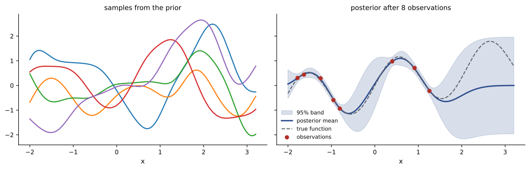
Inputs close together (relative to the length-scale \(\ell\)) have function values that are highly correlated, and inputs far apart are nearly independent. The signal variance \(\sigma_f^2\) sets the typical amplitude of the function. Sampling from the prior makes this concrete: draw a fine grid of inputs, build the covariance matrix, and sample a multivariate Gaussian (Lesson 2). Each sample is a smooth random curve that wiggles on the scale of \(\ell\).
Kernels encode assumptions
Different kernels express different beliefs about the function:
| Kernel | Formula (with \(r = |x - x'|\)) | Functions it produces |
|---|---|---|
| Squared exponential (RBF) | \(\sigma_f^2 e^{-r^2/2\ell^2}\) | infinitely smooth |
| Matérn 5/2 | \(\sigma_f^2(1 + \sqrt5 r/\ell + 5r^2/3\ell^2)e^{-\sqrt5 r/\ell}\) | twice differentiable; often more realistic |
| Matérn 1/2 (exponential) | \(\sigma_f^2 e^{-r/\ell}\) | continuous but rough, like a random walk |
| Periodic | \(\sigma_f^2 \exp\!\left(-2\sin^2(\pi r/p)/\ell^2\right)\) | repeating with period \(p\) |
| Linear | \(\sigma_b^2 + \sigma_v^2 x x'\) | straight lines (Bayesian linear regression) |
| White noise | \(\sigma_n^2\,[x = x']\) | independent noise at each input |
Kernels can be combined. The sum of two kernels models a function that is the sum of two independent processes, such as a smooth trend plus a seasonal cycle. The product of kernels models interactions, such as a periodic pattern whose shape slowly drifts (periodic times RBF). The famous example is the Mauna Loa carbon dioxide record, modeled as a long-term smooth rise plus an annual cycle plus medium-term irregularities plus noise, each a separate kernel. For inputs with several dimensions, an RBF kernel with a separate length-scale for each dimension (automatic relevance determination) learns which inputs matter: a very long length-scale means the function hardly changes along that input.
A valid kernel must produce a positive semidefinite covariance matrix for every set of inputs. Sums and products of valid kernels are valid, which is why building kernels from parts is safe.
Regression with a Gaussian process
Suppose we observe \(y_i = f(x_i) + \varepsilon_i\) with Gaussian noise \(\varepsilon_i \sim \mathcal{N}(0, \sigma_n^2)\), and want to predict \(f\) at new inputs \(X_*\). Under the GP prior, the training outputs and the test function values are jointly Gaussian:
where \(\mathbf{K}\) is the kernel matrix of the training inputs, \(\mathbf{K}_*\) contains the kernel between test and training inputs, and \(\mathbf{K}_{**}\) between test inputs. The Gaussian conditioning formula of Lesson 2 gives the posterior directly:
The posterior mean is a weighted combination of the observed outputs, with weights determined by how strongly each training input correlates with the test input. The posterior variance starts at the prior variance and is reduced by an amount that depends only on where the training inputs are, not on the observed outputs.
Worked problem
One observation
A GP has an RBF kernel with \(\sigma_f = 1\) and \(\ell = 1\), and noise \(\sigma_n = 0.1\). We observe \(y = 2\) at \(x = 0\). Find the posterior mean and standard deviation of \(f\) at \(x = 0\) and at \(x = 1\).
Show solution
- At \(x = 0\): \(k(0, 0) = 1\), so the mean is \(1 \times 2/(1 + 0.01) = 1.98\) and the variance \(1 - 1/1.01 = 0.0099\), standard deviation 0.10.
- At \(x = 1\): \(k(1, 0) = e^{-0.5} = 0.607\). Mean: \(0.607 \times 2/1.01 = 1.20\). Variance: \(1 - 0.607^2/1.01 = 1 - 0.365 = 0.635\), standard deviation 0.80.
Answer: At the observation, the prediction is 1.98 ± 0.10; one length-scale away, 1.20 ± 0.80. The prediction relaxes toward the prior mean of zero and the uncertainty grows with distance from the data.
In practice the matrix inverse is never formed explicitly. The Cholesky factor \(\mathbf{L}\) of \(\mathbf{K} + \sigma_n^2\mathbf{I}\) is computed once, and triangular solves give both the weights and the variances stably.
import numpy as np

rng = np.random.default_rng(2)
f = lambda x: np.sin(3 * x) + 0.3 * x
X = np.sort(rng.uniform(-2, 2, 8))
y = f(X) + rng.normal(0, 0.1, X.size)

def rbf(a, b, ell=0.5, sf=1.0):
    return sf ** 2 * np.exp(-0.5 * (a[:, None] - b[None, :]) ** 2 / ell ** 2)

noise = 0.1
K = rbf(X, X) + noise ** 2 * np.eye(X.size)
L = np.linalg.cholesky(K)                              # stable solves via the Cholesky factor
alpha = np.linalg.solve(L.T, np.linalg.solve(L, y))
Xs = np.array([-1.5, 0.0, 0.7, 3.0])                   # 3.0 is outside the data
Ks = rbf(Xs, X)
mean = Ks @ alpha
v = np.linalg.solve(L, Ks.T)
var = np.diag(rbf(Xs, Xs)) - np.sum(v ** 2, axis=0)
for xs, m, s in zip(Xs, mean, np.sqrt(var)):
print(f"x = {xs:+.1f}: prediction {m:+.2f} +/- {1.96 * s:.2f} (95%), true {f(xs):+.2f}")x = -1.5: prediction +0.52 +/- 0.20 (95%), true +0.53 x = +0.0: prediction +0.08 +/- 0.99 (95%), true +0.00 x = +0.7: prediction +1.05 +/- 0.29 (95%), true +1.07 x = +3.0: prediction -0.00 +/- 1.96 (95%), true +1.31
Near the data the intervals are tight and the predictions accurate. At \(x = 0\), which falls in a gap between observations at −0.81 and 0.40, the interval widens to about ±1. At \(x = 3\), well beyond the data, the prediction returns to the prior mean of zero with the full prior uncertainty: the GP knows that it does not know. This honest uncertainty, growing away from the data, is the property that makes GPs valuable in active learning and optimization. Note also the price: with a stationary kernel and zero mean, a GP cannot extrapolate a trend, so a linear term in the mean or kernel is needed when trends are expected.
Learning hyperparameters
The kernel has hyperparameters (\(\ell\), \(\sigma_f\), \(\sigma_n\), and others for richer kernels). Because the marginal likelihood of a GP is available in closed form, they can be chosen by maximizing it, an instance of empirical Bayes (Lesson 1):
The first term measures data fit and the second penalizes complexity. A very short length-scale lets the function pass through every point (good fit) but spreads prior probability over a vast number of wiggly functions, so the observed data receive little probability (large determinant). A very long length-scale is simple but cannot fit. The marginal likelihood balances the two automatically, a built-in Occam's razor.
import numpy as np

rng = np.random.default_rng(4)
X = np.sort(rng.uniform(0, 10, 40))
y = np.sin(X) + rng.normal(0, 0.2, X.size)

def log_marginal(ell, sf, sn):
    K = sf ** 2 * np.exp(-0.5 * (X[:, None] - X[None, :]) ** 2 / ell ** 2) + sn ** 2 * np.eye(X.size)
    L = np.linalg.cholesky(K)
    a = np.linalg.solve(L.T, np.linalg.solve(L, y))
    fit = -0.5 * y @ a                                  # data fit
    complexity = -np.sum(np.log(np.diag(L)))           # -0.5 log det K: larger for simpler, smoother models
    return fit + complexity - 0.5 * X.size * np.log(2 * np.pi), fit, complexity

for ell in (0.1, 0.3, 1.0, 3.0, 10.0):
    lml, fit, cpx = log_marginal(ell, 1.0, 0.2)
    print(f"length-scale {ell:5.1f}: data fit {fit:8.1f}  complexity term {cpx:6.1f}  log marginal likelihood {lml:7.1f}")

best = max(((log_marginal(l, s, n)[0], l, s, n) for l in np.linspace(0.3, 3, 28)
            for s in (0.5, 1.0, 2.0) for n in (0.05, 0.1, 0.2, 0.4)))
print(f"grid search best: length-scale {best[1]:.1f}, signal sd {best[2]}, noise sd {best[3]} (true noise 0.2)")length-scale 0.1: data fit -11.5 complexity term 12.3 log marginal likelihood -36.0 length-scale 0.3: data fit -12.4 complexity term 26.1 log marginal likelihood -23.0 length-scale 1.0: data fit -15.2 complexity term 44.5 log marginal likelihood -7.5 length-scale 3.0: data fit -36.2 complexity term 54.1 log marginal likelihood -18.9 length-scale 10.0: data fit -198.8 complexity term 58.3 log marginal likelihood -177.3 grid search best: length-scale 1.9, signal sd 1.0, noise sd 0.2 (true noise 0.2)
Short length-scales fit better but pay heavily in the complexity term; the longest length-scale cannot fit a sine wave at all. In practice hyperparameters are optimized with gradients (the derivatives of the log marginal likelihood are available in closed form), using several random restarts because the surface can have multiple optima, each representing a different explanation of the data (for example, a short length-scale with little noise, or a long length-scale with much noise). A fully Bayesian alternative places priors on the hyperparameters and samples them with MCMC (Lesson 7).
Classification and other likelihoods
With a non-Gaussian likelihood the posterior is no longer Gaussian. For binary classification, a latent GP function is passed through a sigmoid, \(p(y = 1 \mid f) = \sigma(f(x))\), as in logistic regression (Lesson 8). The posterior over \(f\) must then be approximated. The Laplace approximation fits a Gaussian at the posterior mode using the curvature there; expectation propagation matches moments site by site and is usually more accurate; variational inference (Lesson 9) optimizes a Gaussian approximation and scales to large data sets. The same machinery handles Poisson likelihoods for counts (for example, the intensity of events over space) and Student-t likelihoods for robust regression.
Scaling to large data
Exact GP regression requires factorizing an \(n \times n\) matrix, costing \(O(n^3)\) time and \(O(n^2)\) memory. A few thousand points are routine; tens of thousands strain a single machine. Several approximations extend the reach:
- Inducing point (sparse) methods summarize the data through \(m \ll n\) pseudo-inputs, reducing cost to \(O(nm^2)\). Stochastic variational versions train on mini-batches and handle millions of points.
- Structured kernel methods exploit grids or Toeplitz structure for fast matrix operations.
- Iterative solvers (conjugate gradients) on GPUs compute the needed solves without forming the Cholesky factor.
- Random features approximate a stationary kernel by a finite set of random cosine features, turning the GP into Bayesian linear regression with \(D\) features.
Inputs with many dimensions pose a different problem: distances become less informative, and a GP with a generic kernel needs a great deal of data. GPs therefore shine for problems with modest numbers of inputs (up to a few dozen) and expensive data, which is exactly the setting of tuning experiments and engineering simulations.
Connections
Gaussian processes connect to several other methods:
- Bayesian linear regression with basis functions \(\boldsymbol\phi(x)\) and prior \(\mathbf{w} \sim \mathcal{N}(\mathbf{0}, \mathbf{I})\) is a GP with kernel \(k(x, x') = \boldsymbol\phi(x)^\top\boldsymbol\phi(x')\). A GP is the limit with infinitely many basis functions, computed without ever listing them (the kernel trick).
- The GP posterior mean equals the prediction of kernel ridge regression with regularization \(\sigma_n^2\); the GP adds the variance.
- A neural network with one hidden layer and random weights becomes a GP as the layer width goes to infinity (Neal, 1994), and the same holds for deep networks; the neural tangent kernel describes the training of very wide networks in the same terms.
- Kriging, developed for estimating ore grades from boreholes, is GP regression with kernels (variograms) fitted to spatial data.
Worked problem
Choosing a kernel for sensor data
Hourly temperature from a building sensor shows a daily cycle whose shape changes slowly over weeks, a gradual seasonal trend, and measurement noise. Propose a kernel.
Show solution
- Seasonal trend: an RBF kernel with a length-scale of weeks to months.
- Daily cycle with drifting shape: a periodic kernel with \(p = 24\) h multiplied by an RBF with a length-scale of a few weeks.
- Noise: a white noise kernel.
Answer: \(k = k_{\text{RBF,long}} + k_{\text{per},24\text{h}} \times k_{\text{RBF,weeks}} + k_{\text{noise}}\), with hyperparameters learned by maximizing the marginal likelihood. Each component can then be plotted separately to interpret the fit.
Common mistakes
MistakeInverting the kernel matrix directly.
InsteadUse a Cholesky factorization and triangular solves, adding a small jitter if needed.
MistakeExpecting a zero-mean stationary GP to extrapolate a trend.
InsteadAdd a linear or polynomial mean or kernel component when trends are expected.
MistakeOptimizing hyperparameters from a single starting point.
InsteadUse several restarts; the marginal likelihood can have multiple optima.
MistakeApplying exact GPs to hundreds of thousands of points.
InsteadUse sparse, variational or iterative approximations.
MistakeIgnoring input scaling.
InsteadStandardize inputs or use per-dimension length-scales so that distances are meaningful.
Summary and key terms
- A GP is a prior over functions: any finite set of values is jointly Gaussian with covariance given by a kernel.
- Kernels encode smoothness, length-scale, periodicity and trends, and can be added and multiplied.
- GP regression uses Gaussian conditioning; uncertainty grows away from the data.
- Hyperparameters are learned by maximizing the closed-form marginal likelihood, which balances fit and complexity.
- Non-Gaussian likelihoods need approximations such as Laplace, expectation propagation or variational inference.
- Exact GPs cost \(O(n^3)\); sparse and iterative methods scale them, and GPs connect to Bayesian linear regression, kernel ridge regression and wide neural networks.
- Gaussian process
- A distribution over functions whose finite marginals are Gaussian.
- Kernel (covariance function)
- The function \(k(x, x')\) giving the covariance between function values.
- Length-scale
- The input distance over which function values remain strongly correlated.
- RBF kernel
- The squared exponential kernel, producing very smooth functions.
- Matérn kernel
- A family of kernels with adjustable smoothness.
- Automatic relevance determination
- Per-input length-scales that reveal which inputs matter.
- Marginal likelihood
- The probability of the data with the function integrated out, used to fit hyperparameters.
- Inducing points
- Pseudo-inputs that summarize the data in sparse GP approximations.
- Kriging
- GP regression as used in geostatistics.
- Kernel trick
- Working with inner products of features through a kernel without computing the features.
Practice problems
Work each problem on paper first, then reveal the answer to check.
RBF kernel with \(\ell = 2\), \(\sigma_f = 1\): covariance between inputs 2 apart?
Show answer
\(e^{-0.5} = 0.61\).
And 6 apart?
Show answer
\(e^{-4.5} = 0.011\).
One observation \(y = 1\) at \(x = 0\), \(\sigma_f = 1\), \(\sigma_n = 0\): posterior mean at a point with \(k = 0.5\)?
Show answer
0.5.
Posterior variance there?
Show answer
\(1 - 0.25 = 0.75\).
Which kernel would model a weekly pattern in sales?
Show answer
A periodic kernel with a period of 7 days (perhaps times an RBF).
What do the two main terms of the GP log marginal likelihood measure?
Show answer
Data fit and model complexity.
Why does a very short length-scale have a poor marginal likelihood?
Show answer
It spreads probability over many wiggly functions, so the observed data get little.
Cost of exact GP regression with \(n\) points?
Show answer
\(O(n^3)\) time, \(O(n^2)\) memory.
GP posterior mean equals the prediction of which method?
Show answer
Kernel ridge regression.
A very long learned length-scale for one input indicates:
Show answer
That input has little effect on the output.
Lesson quiz · 5 questions
Score 60% or more to complete this lesson.
Create a free account to save your progress, take quizzes and earn a certificate.