Information theory: entropy and divergence

In 1948 Claude Shannon, an engineer at Bell Labs, published "A Mathematical Theory of Communication", which defined how to measure information and set the limits on how far data can be compressed and how fast it can be sent over a noisy channel. Shannon's ideas underpin every modem, every compressed file and every fiber link in a data center. They also turned out to be central to machine learning. The loss used to train almost every classifier and every large language model is a quantity from information theory, the cross-entropy; the way models are compared with each other and with data uses the Kullback–Leibler divergence; and the quality of a language model is reported as perplexity, an information-theoretic measure.

This chapter defines information content, entropy, cross-entropy, KL divergence and mutual information, shows how they relate, and connects each to its use in machine learning.

Information content

How much information does learning an outcome give you? Shannon's answer: the less probable the outcome, the more informative it is. The information content (or surprisal) of an outcome with probability \(p\) is

A fair coin flip gives \(-\log_2 0.5 = 1\) bit. Learning which of 8 equally likely outcomes occurred gives 3 bits, because it answers three yes/no questions. An event with probability 1 gives 0 bits: you learn nothing from being told what you already knew. Information from independent events adds, because their probabilities multiply and the logarithm turns products into sums. Using the natural logarithm instead of base 2 measures information in nats (1 nat = 1.443 bits); machine learning code usually works in nats.

Entropy

The entropy of a distribution is its expected information content: how surprised you are, on average, by an outcome drawn from it:

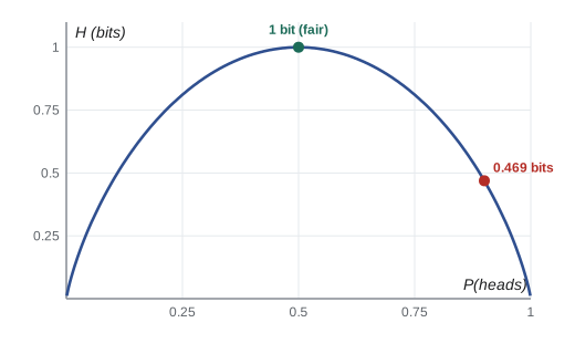
Entropy measures uncertainty. It is zero when one outcome is certain and largest when all outcomes are equally likely: for \(K\) outcomes, the maximum is \(\log_2 K\) bits. Shannon's source coding theorem gives it a concrete meaning: the entropy is the minimum average number of bits per symbol needed to encode messages from the distribution without loss. No compressor can do better.

import numpy as np

def entropy(p):
    p = np.asarray(p, dtype=float)
    p = p[p > 0]                         # 0 log 0 is taken as 0
    return -np.sum(p * np.log2(p)) + 0.0     # + 0.0 turns -0.0 into 0.0

for name, p in [("fair coin", [0.5, 0.5]), ("biased coin", [0.9, 0.1]),
                ("fair die", [1/6] * 6), ("certain", [1.0, 0.0])]:
    print(f"{name:12s} H = {entropy(p):.3f} bits")

fair coin    H = 1.000 bits
biased coin  H = 0.469 bits
fair die     H = 2.585 bits
certain      H = 0.000 bits

Cross-entropy

Suppose the data really come from a distribution \(p\), but we encode or predict them using a model \(q\). The average number of bits needed is the cross-entropy:

It is always at least \(H(p)\), with equality only when \(q = p\): using the wrong distribution costs extra bits. This is exactly the classification loss from Lessons 4 and 6. For a single training example whose true class is \(c\), the target distribution \(p\) is one-hot (1 for class \(c\), 0 elsewhere), and the cross-entropy reduces to \(-\log q(c)\), the negative log-probability the model assigns to the right answer. Averaging over a training set, minimizing cross-entropy is the same as maximizing likelihood.

Kullback–Leibler divergence

The extra cost of using \(q\) instead of \(p\) is the Kullback–Leibler (KL) divergence:

KL divergence is never negative, and it is zero only when the two distributions are identical (Gibbs' inequality). It is a natural measure of how different a model is from the truth. Since \(H(p)\) does not depend on the model, minimizing cross-entropy over \(q\) is the same as minimizing \(D_{\text{KL}}(p\,\|\,q)\).

KL divergence is not a distance in the geometric sense: it is not symmetric, \(D_{\text{KL}}(p\|q) \ne D_{\text{KL}}(q\|p)\) in general, and it does not satisfy the triangle inequality. The asymmetry matters. \(D_{\text{KL}}(p\|q)\) is large wherever \(p\) has probability and \(q\) has very little, so minimizing it forces \(q\) to cover everything \(p\) can do ("mass-covering"). \(D_{\text{KL}}(q\|p)\) penalizes \(q\) for putting probability where \(p\) has little, so minimizing it makes \(q\) concentrate on a high-probability region of \(p\) ("mode-seeking"). Variational inference (AI-320) uses the second form.

import numpy as np

p = np.array([0.6, 0.3, 0.1])            # true distribution
q = np.array([0.4, 0.4, 0.2])            # model distribution

H_p  = -np.sum(p * np.log2(p))
H_pq = -np.sum(p * np.log2(q))           # cross-entropy
KL_pq = np.sum(p * np.log2(p / q))
KL_qp = np.sum(q * np.log2(q / p))
print(f"H(p) = {H_p:.4f}   H(p, q) = {H_pq:.4f} bits")
print(f"KL(p||q) = {KL_pq:.4f} = H(p,q) - H(p) = {H_pq - H_p:.4f}")
print(f"KL(q||p) = {KL_qp:.4f}   (not symmetric)")

H(p) = 1.2955   H(p, q) = 1.4219 bits
KL(p||q) = 0.1265 = H(p,q) - H(p) = 0.1265
KL(q||p) = 0.1320   (not symmetric)

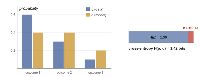
KL divergence appears throughout modern AI: as a regularizer that keeps a fine-tuned language model close to its original (in reinforcement learning from human feedback, a KL penalty stops the model drifting too far), in knowledge distillation (training a small model to match the output distribution of a large one), in variational autoencoders, and in measuring how much a data distribution has shifted between training and deployment.

Perplexity

A language model assigns a probability to each next token. Its cross-entropy on a test text is the average negative log-probability of the tokens that actually occurred. Perplexity is the exponential of that cross-entropy:

It has an intuitive meaning: a perplexity of 20 means the model is, on average, as uncertain as if it were choosing uniformly among 20 tokens. Lower is better. A model guessing uniformly over a vocabulary of 50,000 tokens has a perplexity of 50,000; strong language models reach single-digit perplexities on ordinary text.

import numpy as np

# Probabilities a language model assigned to each actual next token in a short text
probs = np.array([0.40, 0.05, 0.62, 0.21, 0.09, 0.33, 0.71, 0.12])
nll = -np.mean(np.log(probs))            # average cross-entropy in nats per token
print(f"cross-entropy {nll:.3f} nats/token = {nll / np.log(2):.3f} bits/token")
print(f"perplexity {np.exp(nll):.2f}")
print("perplexity of guessing uniformly among 50,000 tokens:", 50_000)

cross-entropy 1.491 nats/token = 2.151 bits/token
perplexity 4.44
perplexity of guessing uniformly among 50,000 tokens: 50000

Perplexity and cross-entropy also connect language modeling to compression: a model with a cross-entropy of 2.15 bits per token could, in principle, compress the text to about 2.15 bits per token using arithmetic coding. Predicting well and compressing well are the same problem.

Mutual information

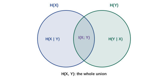
How much does knowing one variable tell you about another? The mutual information between \(X\) and \(Y\) is the reduction in uncertainty about one from learning the other:

It is zero if and only if \(X\) and \(Y\) are independent, and unlike correlation it captures any kind of dependence, not just linear relationships. It is used to select informative features, to build decision trees (where it is called information gain: each split is chosen to reduce the entropy of the labels as much as possible), and in representation learning.

import numpy as np

# Joint distribution of X = "inlet temperature high?" and Y = "fan alarm?"
P = np.array([[0.60, 0.05],             # X = low:  Y = no, yes
              [0.10, 0.25]])            # X = high: Y = no, yes
px, py = P.sum(axis=1), P.sum(axis=0)
H = lambda d: -np.sum(d[d > 0] * np.log2(d[d > 0]))
MI = np.sum(P * np.log2(P / np.outer(px, py)))
print(f"H(X) = {H(px):.3f}, H(Y) = {H(py):.3f}, H(X,Y) = {H(P.ravel()):.3f} bits")
print(f"I(X;Y) = {MI:.3f} bits = H(X) + H(Y) - H(X,Y) = {H(px) + H(py) - H(P.ravel()):.3f}")

H(X) = 0.934, H(Y) = 0.881, H(X,Y) = 1.490 bits
I(X;Y) = 0.325 bits = H(X) + H(Y) - H(X,Y) = 0.325

Label smoothing and calibration

Because cross-entropy rewards pushing the probability of the correct class all the way to 1, models trained with it can become overconfident. Label smoothing replaces the one-hot target with a slightly softened one (for example 0.9 for the correct class and the remaining 0.1 shared among the others), which raises the entropy of the target and discourages extreme confidence. A model is well calibrated when its stated probabilities match observed frequencies: among predictions made with 80% confidence, about 80% should be right. Calibration matters whenever probabilities feed decisions, such as deciding whether to alert an operator or to defer to a human.