High-dimensional geometry, embeddings and kernels

Machine learning lives in spaces of hundreds to tens of thousands of dimensions: an embedding of a sentence, the pixels of an image, the activations of a network layer. Our intuition comes from two and three dimensions, and in high dimensions much of it is wrong. Distances between random points become almost equal, random directions are almost perpendicular, and most of the volume of a ball lies near its surface. This lesson builds the right intuition, shows why it matters for nearest-neighbor search, similarity and clustering, explains how random projections can shrink dimensions while preserving distances, and introduces kernels, which compute inner products in very high-dimensional feature spaces without ever constructing them.

Distances concentrate

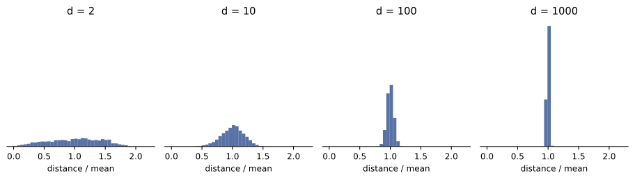
Take random points in a \(d\)-dimensional cube and measure the distance from a query point to each. In two dimensions, the nearest point is much closer than the farthest. As \(d\) grows, the distances bunch together: the ratio of the spread to the nearest distance shrinks toward zero. The reason is the law of large numbers: a squared distance is a sum of \(d\) independent terms, so it concentrates around its mean, with a relative spread proportional to \(1/\sqrt{d}\).

import numpy as np

rng = np.random.default_rng(3)
print("  dim   nearest  farthest  (far - near) / near")
for d in [2, 10, 100, 1000, 10000]:
    pts = rng.uniform(size=(500, d))
    q = rng.uniform(size=d)
    dist = np.linalg.norm(pts - q, axis=1)
    print(f"{d:>5} {dist.min():9.2f} {dist.max():9.2f} {(dist.max() - dist.min()) / dist.min():12.3f}")

  dim   nearest  farthest  (far - near) / near
    2      0.03      1.10       32.308
   10      0.60      2.19        2.651
  100      3.15      4.61        0.462
 1000     12.15     13.74        0.131
10000     40.08     41.31        0.031

This is one face of the curse of dimensionality. If all points are about equally far away, "nearest neighbor" carries little information, and methods built on distance, such as k-nearest neighbors, k-means and kernel smoothing, degrade on raw high-dimensional data. They work in practice because real data is not uniformly random: it lies near lower-dimensional structures (the manifold hypothesis), and learned embeddings are trained so that distances mean something.

Volume lives near the surface

The fraction of a \(d\)-dimensional ball's volume within radius \(1 - \varepsilon\) of its center is \((1 - \varepsilon)^{d}\). For \(d = 1{,}000\) and \(\varepsilon = 0.01\), that is \(0.99^{1000} \approx 4 \times 10^{-5}\): virtually all of the volume is in the outer 1% shell. Likewise, a high-dimensional Gaussian is not concentrated near its mean: samples lie on a thin shell of radius about \(\sigma\sqrt{d}\). Interpolating between two embeddings in a straight line therefore passes through regions where real data never lies, one reason why generative models often interpolate along the sphere instead.

Random directions are nearly orthogonal

The cosine of the angle between two random vectors in \(d\) dimensions has mean zero and standard deviation about \(1/\sqrt{d}\). In three dimensions, random directions are often far from perpendicular; in thousands, they are almost always within a few degrees of 90°.

import numpy as np

rng = np.random.default_rng(4)
for d in [3, 30, 300, 3000]:
    u = rng.normal(size=(2000, d))
    v = rng.normal(size=(2000, d))
    cos = np.sum(u * v, axis=1) / (np.linalg.norm(u, axis=1) * np.linalg.norm(v, axis=1))
    print(f"d = {d:>4}: std of cosine {cos.std():.4f} (1/sqrt(d) = {1 / np.sqrt(d):.4f}), "
          f"fraction with |cos| > 0.1: {np.mean(np.abs(cos) > 0.1):.3f}")

d =    3: std of cosine 0.5858 (1/sqrt(d) = 0.5774), fraction with |cos| > 0.1: 0.909
d =   30: std of cosine 0.1809 (1/sqrt(d) = 0.1826), fraction with |cos| > 0.1: 0.581
d =  300: std of cosine 0.0583 (1/sqrt(d) = 0.0577), fraction with |cos| > 0.1: 0.088
d = 3000: std of cosine 0.0191 (1/sqrt(d) = 0.0183), fraction with |cos| > 0.1: 0.000

This explains several things in modern AI. High-dimensional embedding spaces can hold an enormous number of nearly orthogonal directions, far more than \(d\), which is one hypothesis for how large language models represent many more concepts than they have dimensions ("superposition"). It also tells us how to read similarity scores: in a 3,000-dimensional space, a cosine of 0.1 between unrelated random vectors is already rare, so a cosine of 0.3 indicates a real relationship, while in 30 dimensions it would mean little.

Embeddings and similarity search

An embedding maps an object, such as a word, sentence, image, product or user, to a vector so that similar objects have similar vectors. Embeddings are learned: word2vec and GloVe from co-occurrence statistics, sentence and image embeddings from contrastive training that pulls matching pairs together and pushes others apart, and the internal representations of large language models. Similarity is usually measured by cosine similarity, often by normalizing every vector to unit length so that cosine similarity equals the dot product, and all similarities between two sets can be computed with one matrix product.

import numpy as np

words = ["pump", "chiller", "fan", "breaker", "fuse", "relay", "router", "switch", "firewall"]
rng = np.random.default_rng(6)
topics = rng.normal(size=(3, 64))                       # cooling, electrical, network directions
group = np.repeat([0, 1, 2], 3)
E = topics[group] + 0.6 * rng.normal(size=(9, 64))      # toy 64-dimensional embeddings

E_unit = E / np.linalg.norm(E, axis=1, keepdims=True)  # normalize once
S = E_unit @ E_unit.T                                   # all cosine similarities in one product
for w in ["chiller", "fuse", "router"]:
    k = words.index(w)
    order = np.argsort(-S[k])[1:3]                      # two most similar words, excluding itself
    print(f"{w:>8}: " + ", ".join(f"{words[m]} ({S[k, m]:.2f})" for m in order))

 chiller: fan (0.80), pump (0.79)
    fuse: breaker (0.71), relay (0.70)
  router: switch (0.82), firewall (0.81)

Retrieval-augmented generation, recommendation systems and semantic search all rest on this operation at a much larger scale: find the vectors most similar to a query among millions or billions. Exact search compares the query with every vector, which is too slow at that scale, so vector databases use approximate nearest-neighbor (ANN) indexes, such as graph-based HNSW or clustering-based IVF with product quantization, trading a little recall for speed improvements of hundreds of times.

Random projections

Remarkably, a random linear map can reduce dimension while approximately preserving all pairwise distances. The Johnson–Lindenstrauss lemma states that \(n\) points can be mapped into \(k = O(\log n/\varepsilon^{2})\) dimensions so that every pairwise distance changes by a factor of at most \(1 \pm \varepsilon\), and that a random Gaussian matrix scaled by \(1/\sqrt{k}\) does this with high probability. The required dimension depends on the number of points and the accuracy, not on the original dimension.

import numpy as np

rng = np.random.default_rng(5)
n, d = 300, 10_000
X = rng.normal(size=(n, d))
i, j = rng.integers(0, n, 2000), rng.integers(0, n, 2000)
keep = i != j
i, j = i[keep], j[keep]
orig = np.linalg.norm(X[i] - X[j], axis=1)

for k in [50, 200, 800]:
    R = rng.normal(size=(d, k)) / np.sqrt(k)        # random Gaussian projection
    Y = X @ R
    ratio = np.linalg.norm(Y[i] - Y[j], axis=1) / orig
    print(f"k = {k:>3}: distance ratio mean {ratio.mean():.3f}, 1st-99th percentile "
          f"{np.percentile(ratio, 1):.3f} to {np.percentile(ratio, 99):.3f}")

k =  50: distance ratio mean 0.993, 1st-99th percentile 0.777 to 1.230
k = 200: distance ratio mean 1.000, 1st-99th percentile 0.883 to 1.123
k = 800: distance ratio mean 0.998, 1st-99th percentile 0.941 to 1.054

Distances are preserved on average at every \(k\), and the spread of the distortion shrinks roughly as \(1/\sqrt{k}\). Unlike PCA (Lesson 1), a random projection needs no training data and no SVD, so it is fast and can be applied to streaming data. It underlies sketching algorithms, locality-sensitive hashing for similarity search, and compressed sensing.

Kernels: inner products in feature space

Many algorithms, including support vector machines, ridge regression and PCA, can be written so that the data appear only through inner products \(\mathbf{x}_{i}^{T}\mathbf{x}_{j}\). Replacing each inner product by a kernel function \(k(\mathbf{x}_{i}, \mathbf{x}_{j}) = \phi(\mathbf{x}_{i})^{T}\phi(\mathbf{x}_{j})\) runs the algorithm in the feature space defined by \(\phi\), which may be very high-dimensional or even infinite-dimensional, without ever computing \(\phi\). This is the kernel trick.

• The polynomial kernel \(k(\mathbf{x}, \mathbf{z}) = (\mathbf{x}^{T}\mathbf{z})^{2}\) corresponds to all products of pairs of features.
• The radial basis function (Gaussian) kernel \(k(\mathbf{x}, \mathbf{z}) = \exp(-\|\mathbf{x} - \mathbf{z}\|^{2}/2\ell^{2})\) corresponds to an infinite-dimensional feature space and measures similarity that decays with distance on a length scale \(\ell\).

A function is a valid kernel exactly when every kernel matrix \(K_{ij} = k(\mathbf{x}_{i}, \mathbf{x}_{j})\) it produces is symmetric and positive semidefinite (Mercer's condition).

import numpy as np

x = np.array([1.0, 2.0])
z = np.array([3.0, 1.0])
phi = lambda v: np.array([v[0]**2, np.sqrt(2) * v[0] * v[1], v[1]**2])   # explicit feature map
print("Explicit features:", round(phi(x) @ phi(z), 6), "| kernel (x . z)^2:", (x @ z) ** 2)

rng = np.random.default_rng(7)
P = rng.normal(size=(40, 2))
sq = np.sum(P**2, axis=1)
K = np.exp(-(sq[:, None] + sq[None, :] - 2 * P @ P.T) / 2.0)          # RBF kernel matrix
eig = np.linalg.eigvalsh(K)
print("RBF kernel matrix: symmetric", np.allclose(K, K.T), "| positive semidefinite:", bool(eig.min() > -1e-10))
print("Three largest eigenvalues:", np.round(eig[::-1][:3], 3))

Explicit features: 25.0 | kernel (x . z)^2: 25.0
RBF kernel matrix: symmetric True | positive semidefinite: True
Three largest eigenvalues: [17.572  6.944  5.437]

Kernel matrices are \(n \times n\), so kernel methods become expensive for large \(n\) (memory grows as \(n^{2}\) and solving as \(n^{3}\)), which is one reason deep networks, which learn their features rather than fixing them, took over on large data sets. Kernels remain important in Gaussian processes (Lesson 7), in small-data problems, and as a lens on deep learning: very wide networks trained with small steps behave like kernel machines with a particular kernel, the neural tangent kernel.