Putting it together: models from first principles

This final lesson uses the mathematics of the whole course on two complete models built from scratch. Logistic regression is the simplest probabilistic classifier, and deriving it touches nearly every topic: a probability model (Lesson 6), its likelihood and the cross-entropy loss (Lesson 9), gradients and Hessians (Lesson 4), convexity and Newton's method (Lesson 11), numerical stability (Lesson 5) and evaluation (Lesson 8). A two-layer neural network then shows what changes when the model is no longer linear in its parameters. The aim is to see that the machinery of modern machine learning is not a collection of tricks but a few ideas used consistently.

Step 1: a probability model

For binary labels \(y \in \{0, 1\}\) and features \(\mathbf{x}\), logistic regression models the probability of the positive class as

where \(\mathbf{x}\) includes a constant 1 for the intercept. The score \(z = \mathbf{w}^{T}\mathbf{x}\) is the log-odds: \(\log\frac{p}{1-p} = z\), so each weight says how much its feature raises the log-odds. The decision boundary \(z = 0\) is a hyperplane, which is why logistic regression is a linear classifier.

Step 2: the likelihood and the loss

Each label is a Bernoulli outcome with probability \(p_{i} = \sigma(z_{i})\). The log-likelihood of the data is \(\sum_{i}[y_{i}\log p_{i} + (1 - y_{i})\log(1 - p_{i})]\). Maximizing it (maximum likelihood, Lesson 6) is the same as minimizing its negative, which is the binary cross-entropy between the labels and the predictions (Lesson 9):

The second form, obtained by substituting \(\sigma\) and simplifying, is the one to compute: \(\log(1 + e^{z})\), evaluated with a stable function such as numpy.logaddexp(0, z), never overflows (Lesson 5).

Step 3: gradient and Hessian

Differentiating with the chain rule, using \(\sigma^{\prime}(z) = \sigma(z)(1 - \sigma(z))\), gives remarkably simple results:

The gradient is the prediction error weighted by the features, the same form as for least squares. The Hessian is \(\mathbf{X}^{T}\mathbf{S}\mathbf{X}\) with positive weights, so for any vector \(\mathbf{v}\), \(\mathbf{v}^{T}\mathbf{H}\mathbf{v} = \sum_{i}s_{i}(\mathbf{x}_{i}^{T}\mathbf{v})^{2} \ge 0\): the Hessian is positive semidefinite everywhere and the loss is convex (Lesson 11). There are no bad local minima.

import numpy as np

rng = np.random.default_rng(18)
n = 400
X = rng.normal(size=(n, 2))
w_true, b_true = np.array([2.0, -1.0]), 0.5
p_true = 1 / (1 + np.exp(-(X @ w_true + b_true)))
y = (rng.random(n) < p_true).astype(float)
Xb = np.column_stack([np.ones(n), X])                     # add an intercept column
sigmoid = lambda z: 1 / (1 + np.exp(-z))

def nll(w):                                               # negative log-likelihood (cross-entropy)
    z = Xb @ w
    return np.sum(np.logaddexp(0, z) - y * z)             # stable form of -log likelihood

w = np.array([0.2, 1.0, -0.5])
p = sigmoid(Xb @ w)
g = Xb.T @ (p - y)
H = Xb.T @ (Xb * (p * (1 - p))[:, None])

h = 1e-5
g_num = np.array([(nll(w + h * e) - nll(w - h * e)) / (2 * h) for e in np.eye(3)])
print("Analytic gradient: ", np.round(g, 4))
print("Numerical gradient:", np.round(g_num, 4))
print("Hessian eigenvalues:", np.round(np.linalg.eigvalsh(H), 3), "-> all positive: the problem is convex")

Analytic gradient:  [ -5.784  -35.8724   5.3455]
Numerical gradient: [ -5.784  -35.8724   5.3455]
Hessian eigenvalues: [51.501 77.676 86.01 ] -> all positive: the problem is convex

Step 4: optimization

Because the loss is convex and smooth, both gradient descent and Newton's method find the global minimum. Gradient descent takes small steps along the negative gradient; Newton's method uses the Hessian to jump to the minimum of a local quadratic model, \(\mathbf{w} \leftarrow \mathbf{w} - \mathbf{H}^{-1}\nabla\mathcal{L}\). For logistic regression, each Newton step is a weighted least-squares problem, so the method is also called iteratively reweighted least squares (IRLS).

import numpy as np

rng = np.random.default_rng(18)
n = 400
X = rng.normal(size=(n, 2))
w_true, b_true = np.array([2.0, -1.0]), 0.5
p_true = 1 / (1 + np.exp(-(X @ w_true + b_true)))
y = (rng.random(n) < p_true).astype(float)
Xb = np.column_stack([np.ones(n), X])                     # add an intercept column
sigmoid = lambda z: 1 / (1 + np.exp(-z))

def nll(w):                                               # negative log-likelihood (cross-entropy)
    z = Xb @ w
    return np.sum(np.logaddexp(0, z) - y * z)             # stable form of -log likelihood

w = np.zeros(3)
for step in range(1, 2001):                               # gradient descent
    grad = Xb.T @ (sigmoid(Xb @ w) - y)
    w -= 0.01 * grad
    if step in (10, 100, 2000):
        print(f"GD step {step:>4}: NLL {nll(w):.4f}, w = {np.round(w, 3)}")

w = np.zeros(3)
for it in range(1, 7):                                    # Newton method (IRLS)
    p = sigmoid(Xb @ w)
    H = Xb.T @ (Xb * (p * (1 - p))[:, None])
    w -= np.linalg.solve(H, Xb.T @ (p - y))
    print(f"Newton iteration {it}: NLL {nll(w):.6f}")
print("Newton solution:", np.round(w, 3), "| true (b, w1, w2): [0.5, 2.0, -1.0]")

GD step   10: NLL 174.9172, w = [ 0.402  1.961 -0.735]
GD step  100: NLL 174.8455, w = [ 0.421  2.039 -0.759]
GD step 2000: NLL 174.8455, w = [ 0.421  2.039 -0.759]
Newton iteration 1: NLL 187.252710
Newton iteration 2: NLL 175.933003
Newton iteration 3: NLL 174.860961
Newton iteration 4: NLL 174.845531
Newton iteration 5: NLL 174.845527
Newton iteration 6: NLL 174.845527
Newton solution: [ 0.421  2.039 -0.759] | true (b, w1, w2): [0.5, 2.0, -1.0]

Newton's method converges to six-figure accuracy in five iterations, showing its quadratic convergence near the optimum; gradient descent takes about a hundred steps to reach the same loss. Both recover weights close to the true values (0.5, 2.0, −1.0), with the differences due to the randomness of 400 samples. For millions of features, the \(d \times d\) Hessian becomes too expensive and first-order methods win; for a few hundred features, Newton's method is hard to beat.

Step 5: evaluation and interpretation

A probabilistic model should be judged not only on accuracy but on the quality of its probabilities. Cross-entropy on held-out data measures how much the model reduces uncertainty compared with a baseline that ignores the features; the difference is the information the features provide, in nats per example (Lesson 9). Calibration asks whether predicted probabilities match observed frequencies: among examples predicted at about 70%, about 70% should be positive.

import numpy as np

rng = np.random.default_rng(18)
n = 400
X = rng.normal(size=(n, 2))
w_true, b_true = np.array([2.0, -1.0]), 0.5
p_true = 1 / (1 + np.exp(-(X @ w_true + b_true)))
y = (rng.random(n) < p_true).astype(float)
Xb = np.column_stack([np.ones(n), X])                     # add an intercept column
sigmoid = lambda z: 1 / (1 + np.exp(-z))

def nll(w):                                               # negative log-likelihood (cross-entropy)
    z = Xb @ w
    return np.sum(np.logaddexp(0, z) - y * z)             # stable form of -log likelihood

w = np.zeros(3)
for _ in range(8):
    p = sigmoid(Xb @ w)
    w -= np.linalg.solve(Xb.T @ (Xb * (p * (1 - p))[:, None]), Xb.T @ (p - y))
p = sigmoid(Xb @ w)

ce = nll(w) / n
base = y.mean()
ce_base = -(base * np.log(base) + (1 - base) * np.log(1 - base))
print(f"Cross-entropy per example: model {ce:.3f} nats, predict-the-base-rate {ce_base:.3f} nats")
print(f"Information gained from the features: {ce_base - ce:.3f} nats per example")

bins = np.digitize(p, [0.2, 0.4, 0.6, 0.8])
print("Calibration (predicted vs observed rate of y = 1 by bin):")
for b in range(5):
    m = bins == b
    print(f"  bin {b}: n = {m.sum():>3}, predicted {p[m].mean():.2f}, observed {y[m].mean():.2f}")

Cross-entropy per example: model 0.437 nats, predict-the-base-rate 0.688 nats
Information gained from the features: 0.251 nats per example
Calibration (predicted vs observed rate of y = 1 by bin):
  bin 0: n =  87, predicted 0.10, observed 0.06
  bin 1: n =  55, predicted 0.29, observed 0.38
  bin 2: n =  63, predicted 0.51, observed 0.54
  bin 3: n =  73, predicted 0.70, observed 0.67
  bin 4: n = 122, predicted 0.93, observed 0.92

The features reduce the cross-entropy from 0.688 to 0.437 nats per example, about 0.25 nats of information each. The calibration table shows predicted and observed rates agreeing to within sampling error in every bin, as expected for a correctly specified model fitted by maximum likelihood. (Evaluated on its own training data, as here for brevity, the agreement is slightly flattering; Lesson 8 explains why a held-out set is needed for an honest assessment.)

Step 6: beyond linear models

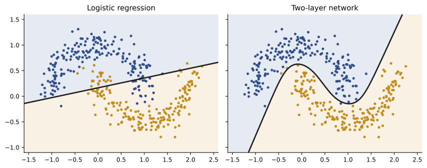
When the classes cannot be separated by a hyperplane, logistic regression on the raw features fails however well it is optimized: its bias is the problem (Lesson 8). A neural network replaces the fixed features with learned ones. A two-layer network computes hidden features \(\mathbf{a} = \tanh(\mathbf{W}_{1}^{T}\mathbf{x} + \mathbf{b}_{1})\) and then performs logistic regression on them: \(p = \sigma(\mathbf{w}_{2}^{T}\mathbf{a} + b_{2})\). Training uses the same cross-entropy loss, with gradients from backpropagation (Lessons 4 and 5). The output layer's gradient is again "prediction minus label" times the hidden features; it is then passed back through \(\mathbf{w}_{2}\) and the derivative of tanh, \(1 - a^{2}\), to the first layer.

import numpy as np

rng = np.random.default_rng(19)
def moons(n):
    t = rng.uniform(0, np.pi, n)
    top = np.column_stack([np.cos(t), np.sin(t)])
    bottom = np.column_stack([1 - np.cos(t), 0.5 - np.sin(t)])
    X = np.vstack([top, bottom]) + rng.normal(0, 0.15, (2 * n, 2))
    return X, np.r_[np.zeros(n), np.ones(n)]
Xtr, ytr = moons(200)
Xte, yte = moons(500)

H = 16
W1 = rng.normal(0, 1, (2, H)); b1 = np.zeros(H)
W2 = rng.normal(0, 1 / np.sqrt(H), H); b2 = 0.0
lr, lam = 0.5, 1e-3
for epoch in range(3000):
    Z = Xtr @ W1 + b1; A = np.tanh(Z)                    # forward
    p = 1 / (1 + np.exp(-(A @ W2 + b2)))
    d_out = (p - ytr) / ytr.size                        # backward: gradient of mean cross-entropy
    gW2 = A.T @ d_out + lam * W2; gb2 = d_out.sum()
    dA = np.outer(d_out, W2) * (1 - A**2)
    gW1 = Xtr.T @ dA + lam * W1; gb1 = dA.sum(axis=0)
    W1 -= lr * gW1; b1 -= lr * gb1; W2 -= lr * gW2; b2 -= lr * gb2

def acc(X, y):
    p = 1 / (1 + np.exp(-(np.tanh(X @ W1 + b1) @ W2 + b2)))
    return np.mean((p > 0.5) == y)

Xb = np.column_stack([np.ones(len(Xtr)), Xtr]); w = np.zeros(3)
for _ in range(5000):                                   # logistic regression baseline
    w -= 0.5 * Xb.T @ (1 / (1 + np.exp(-Xb @ w)) - ytr) / len(ytr)
lin_acc = np.mean(((np.column_stack([np.ones(len(Xte)), Xte]) @ w) > 0) == yte)
print(f"Logistic regression test accuracy: {lin_acc:.3f}")
print(f"Two-layer network: train accuracy {acc(Xtr, ytr):.3f}, test accuracy {acc(Xte, yte):.3f}")

Logistic regression test accuracy: 0.866
Two-layer network: train accuracy 0.993, test accuracy 0.990

The network reaches 99% test accuracy where the linear model is stuck near 87%. What the network gains in flexibility it loses in guarantees: its loss is no longer convex in the parameters, different random initializations give different solutions, and the step size, width, regularization and number of epochs must be chosen by validation rather than by theory. Those are the trade-offs studied in the courses that follow: optimization for machine learning (AI-310), probabilistic models (AI-320), and the deep learning of language (AI-340) and vision (AI-350).

The common thread

Every model in this course, and nearly every model in modern AI, is built the same way: choose a parameterized family of functions (linear algebra), turn the data into a likelihood or loss (probability and information theory), compute its gradient (calculus and automatic differentiation), minimize it (optimization), and measure how well the result generalizes (learning theory). Large language models replace the two-moons data with trillions of tokens and the 65 parameters with hundreds of billions, but the cross-entropy loss, the backpropagated gradients, the low-precision matrix products and the held-out evaluations are the same mathematics you have now worked through.