
AI-210 · Lesson 6 of 12 · 33 min
Probability for learning
Machine learning is learning from data that is noisy, incomplete and drawn from a world we never see in full. Probability is the language for reasoning about that uncertainty. It explains what a model is really doing when it fits data (maximizing a likelihood), why a classifier's outputs can be read as probabilities, where loss functions come from, why regularization works (it is a prior belief), and how to update beliefs when new evidence arrives. Large language models are, at their core, probability distributions over the next word.
This chapter reviews random variables, expectation, variance and the common distributions, then covers the three ideas machine learning uses most: Bayes' rule, maximum likelihood estimation and maximum a posteriori estimation. It shows how familiar loss functions such as squared error and cross-entropy fall out of probability, and how a prior becomes a regularizer.
Random variables and distributions
A random variable assigns a number to each outcome of an uncertain process. A discrete random variable, such as the roll of a die or the class of an image, has a probability mass function \(P(X = x)\) whose values sum to 1. A continuous random variable, such as a temperature or a sensor reading, has a probability density function \(p(x)\) whose integral over all values is 1; probabilities are areas under the density, so \(P(a \le X \le b) = \int_a^b p(x)\,dx\), and a density can exceed 1.
For two variables, the joint distribution \(p(x, y)\) describes them together. Summing or integrating out one variable gives the marginal, \(p(x) = \sum_y p(x, y)\). The conditional distribution \(p(y \mid x) = p(x, y)/p(x)\) describes \(y\) once \(x\) is known, and rearranging gives the product rule, \(p(x, y) = p(y \mid x)\,p(x)\). Variables are independent when \(p(x, y) = p(x)p(y)\): knowing one tells you nothing about the other. Supervised learning is, at bottom, estimating a conditional distribution \(p(y \mid \mathbf{x})\): the label given the features.
Expectation and variance
The expectation (mean) of a random variable is its probability-weighted average, \(\mathbb{E}[X] = \sum_x x\,P(x)\) or \(\int x\,p(x)\,dx\). Expectation is linear: \(\mathbb{E}[aX + bY] = a\mathbb{E}[X] + b\mathbb{E}[Y]\), whether or not \(X\) and \(Y\) are independent. The variance measures spread around the mean:
and the standard deviation is its square root. For two variables, the covariance \(\operatorname{Cov}(X, Y) = \mathbb{E}[(X - \mathbb{E}X)(Y - \mathbb{E}Y)]\) measures how they vary together, and the correlation divides it by both standard deviations to give a value between −1 and 1. For a vector of variables, the covariance matrix collects all pairwise covariances; it is symmetric and positive semidefinite, which is why PCA (Lesson 1) can diagonalize it.
Worked problem
Mean and variance of a die
Find the expectation and variance of the roll of a fair six-sided die.
Show solution
- \(\mathbb{E}[X] = (1 + 2 + 3 + 4 + 5 + 6)/6 = 3.5\).
- \(\mathbb{E}[X^2] = (1 + 4 + 9 + 16 + 25 + 36)/6 = 91/6 = 15.17\).
- \(\operatorname{Var}(X) = 15.17 - 3.5^2 = 2.917\), so the standard deviation is 1.708.
Answer: Mean 3.5 and variance 35/12 ≈ 2.92. The mean is not a value the die can show, which is normal: an expectation is an average, not a likely outcome.
Averages of many independent samples settle toward the expectation (the law of large numbers), and their fluctuations shrink in proportion to \(1/\sqrt{n}\). This is why more data gives more reliable estimates, and why a test set of 100 examples gives a much noisier accuracy figure than one of 10,000.
import numpy as np

rng = np.random.default_rng(7)
rolls = rng.integers(1, 7, size=100_000)          # fair six-sided die
for n in (10, 100, 1000, 100_000):
    print(f"n = {n:>6}: sample mean {rolls[:n].mean():.4f}")
print("expected value 3.5, variance", round(np.var(np.arange(1, 7)), 4))n = 10: sample mean 4.1000 n = 100: sample mean 3.6900 n = 1000: sample mean 3.5750 n = 100000: sample mean 3.5071 expected value 3.5, variance 2.9167
Common distributions
- Bernoulli: a single yes/no outcome with \(P(X = 1) = \theta\). Mean \(\theta\), variance \(\theta(1 - \theta)\). Binary classification models output a Bernoulli parameter.
- Categorical: one of \(K\) outcomes with probabilities \(\theta_1, \dots, \theta_K\) summing to 1. Multi-class classifiers and language models output categorical distributions (via softmax).
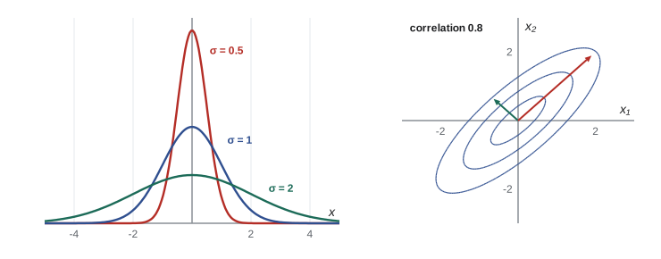
- Gaussian (normal): density \(\mathcal{N}(x; \mu, \sigma^2) = \dfrac{1}{\sqrt{2\pi\sigma^2}}\exp\!\left(-\dfrac{(x - \mu)^2}{2\sigma^2}\right)\). By the central limit theorem, sums of many small independent effects are approximately Gaussian, which makes it the default model for measurement noise.
- Multivariate Gaussian: \(\mathcal{N}(\mathbf{x}; \boldsymbol{\mu}, \boldsymbol{\Sigma})\) with mean vector \(\boldsymbol{\mu}\) and covariance matrix \(\boldsymbol{\Sigma}\). Its contours are ellipses whose axes are the eigenvectors of \(\boldsymbol{\Sigma}\).
- Uniform, Poisson (counts of events, such as requests per second) and Beta (a distribution over a probability, used as a prior below) complete the everyday toolkit.
Bayes' rule
Combining the product rule in both orders gives Bayes' rule, which turns the probability of evidence given a hypothesis into the probability of the hypothesis given the evidence:
\(P(H)\) is the prior, our belief before seeing the evidence; \(P(E \mid H)\) is the likelihood; and \(P(H \mid E)\) is the posterior. The denominator, the evidence, normalizes the result.
Worked problem
A fault detector
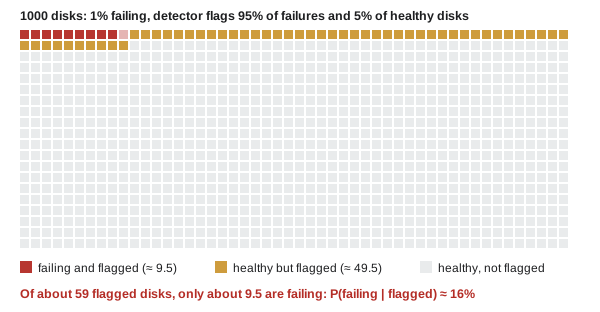
A model monitors servers for an impending disk failure. 1% of disks are actually failing. The model flags 95% of failing disks, and wrongly flags 5% of healthy ones. If a disk is flagged, what is the probability that it is really failing?
Show solution
- Prior: \(P(F) = 0.01\). Likelihoods: \(P(\text{flag} \mid F) = 0.95\), \(P(\text{flag} \mid \text{healthy}) = 0.05\).
- Evidence: \(P(\text{flag}) = 0.95 \times 0.01 + 0.05 \times 0.99 = 0.0095 + 0.0495 = 0.059\).
- Posterior: \(P(F \mid \text{flag}) = 0.0095/0.059 = 0.161\).
Answer: Only about 16%. Because failures are rare, the 5% false-positive rate on the many healthy disks produces five times as many false alarms as true detections. This base-rate effect is why accuracy alone is a misleading measure for rare-event detection, and why precision and recall (AI-230) matter.
Maximum likelihood estimation
A probabilistic model has parameters \(\boldsymbol{\theta}\), and assigns a probability (or density) to each observation. Given independent observations \(x_1, \dots, x_N\), the likelihood is the probability of the whole data set as a function of the parameters, and maximum likelihood estimation (MLE) chooses the parameters that make the observed data most probable. Because products of many small numbers underflow and are awkward to differentiate, we maximize the log-likelihood instead (the logarithm is increasing, so the maximizer is the same):
Equivalently, MLE minimizes the negative log-likelihood (NLL), and that is exactly what most machine learning loss functions are.
Worked problem
MLE for a coin
A coin lands heads 7 times in 10 flips. Find the maximum likelihood estimate of \(\theta = P(\text{heads})\).
Show solution
- Log-likelihood: \(\ell(\theta) = 7\log\theta + 3\log(1 - \theta)\).
- \(d\ell/d\theta = 7/\theta - 3/(1 - \theta) = 0\), so \(7(1 - \theta) = 3\theta\) and \(\theta = 0.7\).
Answer: \(\hat{\theta} = 0.7\): the observed fraction. In general the MLE of a Bernoulli or categorical probability is the observed frequency.
For a Gaussian, maximizing the log-likelihood gives the sample mean for \(\mu\) and the average squared deviation (dividing by \(N\), not \(N - 1\)) for \(\sigma^2\). The MLE of the variance is slightly biased low; the familiar \(N - 1\) version corrects that.
import numpy as np

rng = np.random.default_rng(3)
x = rng.normal(loc=24.0, scale=1.5, size=200)    # 200 temperature readings

mu_hat = x.mean()                                # maximum likelihood estimate of the mean
var_mle = ((x - mu_hat) ** 2).mean()             # MLE of the variance (divides by N)
var_unb = x.var(ddof=1)                          # unbiased estimate (divides by N - 1)
print(f"mean {mu_hat:.3f}   MLE variance {var_mle:.3f}   unbiased {var_unb:.3f}")

def loglik(mu, sigma):
    return np.sum(-0.5 * np.log(2 * np.pi * sigma**2) - (x - mu)**2 / (2 * sigma**2))

for mu in (23.0, mu_hat, 25.0):
print(f"log-likelihood at mu = {mu:.3f}: {loglik(mu, np.sqrt(var_mle)):.2f}")mean 24.072 MLE variance 2.387 unbiased 2.399 log-likelihood at mu = 23.000: -418.99 log-likelihood at mu = 24.072: -370.81 log-likelihood at mu = 25.000: -406.84
Where loss functions come from
Two of the most common losses are negative log-likelihoods in disguise:
- Squared error. If a regression model predicts \(\hat{y} = f(\mathbf{x})\) and assumes Gaussian noise, \(y \sim \mathcal{N}(f(\mathbf{x}), \sigma^2)\), the negative log-likelihood of the data is \(\sum (y_i - f(\mathbf{x}_i))^2/(2\sigma^2)\) plus a constant. Minimizing squared error is maximum likelihood under Gaussian noise.
- Cross-entropy. If a classifier outputs a categorical distribution \(\mathbf{p}\) over classes, the negative log-likelihood of the true class \(c\) is \(-\log p_c\), exactly the cross-entropy loss of Lesson 4. Training a language model to predict the next token is maximum likelihood estimation of a categorical distribution over its vocabulary.
Knowing this tells you when a loss is appropriate. Squared error assumes symmetric, Gaussian-like noise and is sensitive to outliers; if errors have heavy tails, a loss derived from a heavier-tailed distribution (such as the absolute error from a Laplace distribution) may suit the data better.
Maximum a posteriori estimation and priors
MLE trusts the data completely. With little data, that can go badly: a coin that lands heads 3 times in 3 flips has an MLE of \(\theta = 1\), claiming tails is impossible. Bayesian reasoning adds a prior \(p(\boldsymbol{\theta})\) expressing beliefs before the data, and the maximum a posteriori (MAP) estimate maximizes the posterior:
For a coin, a convenient prior is the Beta(\(a\), \(b\)) distribution, which acts like \(a - 1\) imaginary heads and \(b - 1\) imaginary tails added to the data.
heads, n = 7, 10
mle = heads / n                                   # maximum likelihood
a, b = 2, 2                                       # Beta(2, 2) prior: a mild belief in fairness
map_est = (heads + a - 1) / (n + a + b - 2)       # maximum a posteriori
post_mean = (heads + a) / (n + a + b)             # posterior mean
print(f"MLE {mle:.3f}  MAP {map_est:.3f}  posterior mean {post_mean:.3f}")

heads, n = 700, 1000                              # same ratio, much more data
print(f"with 1000 flips: MLE {heads / n:.3f} MAP {(heads + a - 1) / (n + a + b - 2):.3f}")MLE 0.700 MAP 0.667 posterior mean 0.643 with 1000 flips: MLE 0.700 MAP 0.700
With 10 flips the prior pulls the estimate toward 0.5; with 1000 flips the data overwhelms it and MAP agrees with MLE. That is the general pattern: priors matter most when data is scarce.
Regularization is a prior
In models with many parameters, MAP estimation has a direct interpretation. Suppose each weight has a Gaussian prior with mean 0 and variance \(\tau^2\): we believe weights are probably small. Then \(-\log p(\mathbf{w}) = \|\mathbf{w}\|^2/(2\tau^2)\) plus a constant, and the MAP objective becomes
which is exactly L2 regularization (weight decay, or ridge regression). A Laplace prior gives L1 regularization (the lasso), which pushes many weights to exactly zero. Regularization, introduced in AI-101 as a defense against overfitting, is a statement of prior belief, and its strength \(\lambda\) is how firmly that belief is held relative to the data.
Worked problem
Ridge regression as MAP
A linear model has Gaussian noise with \(\sigma = 2\) and a Gaussian prior on its weights with \(\tau = 0.5\). What L2 regularization strength corresponds to this MAP estimate (with the loss written as a sum of squared errors)?
Show solution
- Negative log-posterior: \(\sum(y_i - \mathbf{w}^\top\mathbf{x}_i)^2/(2\sigma^2) + \|\mathbf{w}\|^2/(2\tau^2)\).
- Multiply by \(2\sigma^2\): \(\sum(y_i - \mathbf{w}^\top\mathbf{x}_i)^2 + (\sigma^2/\tau^2)\|\mathbf{w}\|^2\).
- \(\lambda = 4/0.25 = 16\).
Answer: \(\lambda = 16\). Noisier data (larger \(\sigma\)) or a stronger belief that weights are small (smaller \(\tau\)) both increase regularization.
Beyond point estimates
Lesson 7 extends these ideas to vectors with the multivariate Gaussian, where Bayesian estimates can be computed exactly.
MLE and MAP give a single best value of the parameters. Fully Bayesian methods keep the whole posterior distribution, which expresses how uncertain the parameters are, and average predictions over it. This gives honest uncertainty estimates, valuable when decisions are costly, but the posterior is rarely computable exactly for large models. Approximations such as sampling (Markov chain Monte Carlo) and variational inference, covered in AI-320, make it practical for many models, and ideas such as ensembles and dropout at test time approximate it cheaply for neural networks.
Common mistakes
MistakeIgnoring the base rate when interpreting a positive test or alarm.
InsteadUse Bayes' rule: with rare events, most positives can be false even for an accurate detector.
MistakeConfusing \(P(E \mid H)\) with \(P(H \mid E)\).
InsteadThey differ by the ratio of priors; Bayes' rule converts one into the other.
MistakeReading a probability density value as a probability.
InsteadProbabilities are areas under the density; density values can exceed 1.
MistakeMultiplying many small probabilities directly.
InsteadSum log-probabilities to avoid underflow.
MistakeTreating regularization as an unexplained trick.
InsteadIt is a prior on the weights: L2 corresponds to a Gaussian prior, L1 to a Laplace prior.
Summary and key terms
- Random variables have mass functions (discrete) or densities (continuous); joint, marginal and conditional distributions are linked by the product rule.
- Expectation is linear; variance \(= \mathbb{E}[X^2] - \mathbb{E}[X]^2\); covariance matrices are symmetric and positive semidefinite.
- Sample means converge to the expectation, with errors shrinking like \(1/\sqrt{n}\).
- Bernoulli, categorical and Gaussian distributions are the workhorses of machine learning.
- Bayes' rule: posterior ∝ likelihood × prior; base rates matter enormously for rare events.
- MLE maximizes the log-likelihood; squared error is Gaussian MLE and cross-entropy is categorical MLE.
- MAP adds a log-prior; priors matter most with little data.
- L2 regularization is a Gaussian prior on weights, L1 a Laplace prior, with \(\lambda = \sigma^2/\tau^2\).
- Random variable
- A quantity whose value depends on the outcome of an uncertain process.
- Probability density
- A function whose integral over an interval gives the probability of that interval.
- Marginal distribution
- The distribution of one variable obtained by summing or integrating out others.
- Conditional distribution
- The distribution of one variable given the value of another.
- Independence
- The property that \(p(x, y) = p(x)p(y)\).
- Expectation
- The probability-weighted average of a random variable.
- Variance
- The expected squared deviation from the mean.
- Covariance matrix
- The matrix of covariances between all pairs of components of a random vector.
- Gaussian distribution
- The normal distribution, with a bell-shaped density defined by a mean and variance.
- Prior
- A probability distribution expressing beliefs before seeing data.
- Likelihood
- The probability of the observed data as a function of the parameters.
- Posterior
- The probability distribution of parameters or hypotheses after seeing data.
- Maximum likelihood estimation
- Choosing parameters that maximize the probability of the observed data.
- MAP estimation
- Choosing parameters that maximize the posterior probability.
- Negative log-likelihood
- The negative of the log-likelihood, minimized as a loss function.
- Base rate
- The prior frequency of an event in the population.
Practice problems
Work each problem on paper first, then reveal the answer to check.
A random variable takes values 0, 1 and 2 with probabilities 0.5, 0.3 and 0.2. Find its mean and variance.
Show answer
E[X] = 0.3 + 0.4 = 0.7; E[X²] = 0.3 + 0.8 = 1.1; Var = 1.1 − 0.49 = 0.61.
If Var(X) = 4 and Var(Y) = 9 and X and Y are independent, what is Var(2X − Y)?
Show answer
4 × 4 + 9 = 25 (variances of independent variables add; constants are squared).
What is the variance of a Bernoulli variable with θ = 0.2, and at what θ is it largest?
Show answer
0.2 × 0.8 = 0.16; it is largest (0.25) at θ = 0.5.
A test for a rare condition (prevalence 0.1%) has 99% sensitivity and a 1% false-positive rate. What is P(condition | positive)?
Show answer
0.99 × 0.001/(0.99 × 0.001 + 0.01 × 0.999) = 0.00099/0.01098 = 9.0%.
A die is rolled 60 times and shows a six 15 times. What is the MLE of P(six)?
Show answer
15/60 = 0.25.
With a Beta(3, 3) prior, what is the MAP estimate for 2 heads in 2 flips?
Show answer
(2 + 3 − 1)/(2 + 3 + 3 − 2) = 4/6 = 0.667, compared with an MLE of 1.
Write the negative log-likelihood of observations \(y_i\) under \(\mathcal{N}(\mu, 1)\), and find the minimizing \(\mu\).
Show answer
NLL = Σ(yᵢ − μ)²/2 + constant; setting the derivative to zero gives μ = mean of the yᵢ.
A classifier assigns probability 0.25 to the correct class. What is the cross-entropy loss for that example (natural log)?
Show answer
−ln 0.25 = 1.386.
Noise has σ = 1 and the weight prior has τ = 0.1. What is λ in the equivalent ridge regression?
Show answer
λ = σ²/τ² = 1/0.01 = 100: a strong pull toward small weights.
An accuracy of 90% is measured on 100 test examples. Roughly how large is its standard error, and how many examples would halve it?
Show answer
√(0.9 × 0.1/100) = 0.03 (3 points); four times as many examples (400) halves it.
Lesson quiz · 5 questions
Score 60% or more to complete this lesson.
Create a free account to save your progress, take quizzes and earn a certificate.